How to Tackle Time Series Assignments Using ARIMA and SARIMA Models

Understanding Time Series Data

Time series data consists of observations recorded at consistent time intervals, such as daily, monthly, or yearly. Unlike cross-sectional data, which captures a single point in time, time series data tracks changes over a period, making it valuable for trend analysis and forecasting.

Key Characteristics of Time Series Data

Time series data is composed of four primary components:

• Trend – A long-term upward or downward movement in the data. For example, a company’s sales might show a steady increase over several years.
• Seasonality – Regular, repeating patterns tied to specific time periods (e.g., higher ice cream sales in summer or retail spikes during holidays).
• Cyclical Patterns – Fluctuations that occur at irregular intervals, often influenced by economic cycles (e.g., recessions and booms).
• Random Noise (Irregular Component) – Unpredictable variations caused by external factors or measurement errors.

Understanding these components helps in decomposing time series data, making it easier to analyze and model.

Common Applications of Time Series Analysis

• Finance & Economics – Stock price movements, GDP growth, inflation rates.
• Healthcare – Patient vital sign monitoring, disease outbreak tracking.
• Retail & E-commerce – Sales forecasting, inventory management.
• Environmental Science – Weather prediction, pollution level analysis.
• Manufacturing – Equipment failure prediction, quality control.

Given its broad applicability, mastering time series techniques is highly beneficial for students pursuing careers in data science, economics, or business analytics.

Key Techniques in Time Series Analysis

Analyzing time series data involves several statistical methods, broadly categorized into descriptive and predictive techniques.

Descriptive Time Series Analysis

Descriptive techniques summarize historical data to uncover patterns and trends.

Moving Averages

Moving averages smooth out short-term fluctuations, making long-term trends more visible. Common types include:

• Simple Moving Average (SMA) – Average of past 'n' observations.
• Weighted Moving Average (WMA) – Assigns different weights to past data points.
• Exponential Moving Average (EMA) – Gives more importance to recent observations.

Time Series Decomposition

This method breaks down a time series into its core components:

• Additive Model – Used when seasonal variations are constant over time.
• Multiplicative Model – Used when seasonal fluctuations change with trend magnitude.

Decomposition helps isolate trends and seasonality, making further analysis more manageable.

Predictive Time Series Analysis

Predictive techniques forecast future values based on historical patterns.

Autoregressive (AR) Models

AR models predict future values using a linear combination of past values. For example, an AR(1) model uses the immediately preceding observation:

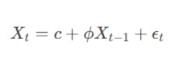
where ϕ is the coefficient and ϵt is white noise.

Moving Average (MA) Models

MA models use past forecast errors to predict future values. An MA(1) model can be written as:

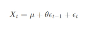
where θ is the coefficient of the error term.

These models are often combined into ARMA (Autoregressive Moving Average) models for better forecasting accuracy.

Popular Models for Time Series Forecasting

Several advanced models are used depending on data characteristics.

ARIMA Model (Autoregressive Integrated Moving Average)

ARIMA is one of the most widely used models for non-seasonal time series forecasting. It consists of three components:

• AR (Autoregression) – Captures the relationship between past and current values.
• I (Integrated) – Uses differencing to make the data stationary (removing trend).
• MA (Moving Average) – Accounts for past error terms in predictions.

An ARIMA model is denoted as ARIMA(p, d, q), where:

• p = Number of autoregressive terms
• d = Degree of differencing
• q = Number of moving average terms

Steps to Build an ARIMA Model

• Check Stationarity – Use the Augmented Dickey-Fuller (ADF) test.
• Differencing – If non-stationary, apply differencing (d).
• Identify AR MA Terms – Use ACF and PACF plots.
• Model Estimation Validation – Compare models using AIC/BIC.

SARIMA Model (Seasonal ARIMA)

SARIMA extends ARIMA to handle seasonal patterns. It is denoted as SARIMA(p, d, q)(P, D, Q, s), where:

(P, D, Q) = Seasonal AR, differencing, and MA terms

s = Seasonal period (e.g., 12 for monthly data)

SARIMA is useful for datasets with recurring patterns, such as monthly sales or quarterly economic data.

Challenges in Time Series Analysis

Despite its usefulness, time series analysis presents several challenges that students should be aware of.

Handling Non-Stationary Data

Many time series datasets exhibit trends or seasonality, violating the stationarity assumption required for many models.

Differencing

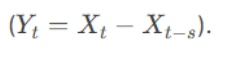
• First Differencing – Subtracts each observation from the previous one
• Seasonal Differencing – Used for seasonal patterns

Transformations

• Log Transformation – Stabilizes variance in exponential growth data.
• Box-Cox Transformation – Generalizes log and power transformations.

Selecting the Right Model

Choosing the best forecasting model requires careful evaluation.

ACF and PACF Plots

• Autocorrelation Function (ACF) – Helps identify MA terms.
• Partial Autocorrelation Function (PACF) – Helps identify AR terms.

Model Evaluation Metrics

• Mean Absolute Error (MAE) – Average absolute forecast error.
• Root Mean Squared Error (RMSE) – Penalizes larger errors more heavily.
• AIC/BIC – Balances model fit and complexity.

Conclusion

Time series analysis serves as an essential statistical tool for examining data patterns over time and generating accurate future forecasts. By developing a strong grasp of fundamental concepts—including trend decomposition, ARIMA modeling, and seasonal SARIMA adjustments—students can confidently approach and solve complex statistics assignments that involve time-dependent datasets.

Key insights to remember:

• Time series data consists of four primary elements: trend, seasonality, cyclical patterns, and random noise, each requiring careful analysis.
• Descriptive techniques such as moving averages and time series decomposition help summarize historical data and identify underlying patterns.
• Predictive modeling approaches, particularly ARIMA and SARIMA, provide robust frameworks for forecasting future values with precision.
• A major challenge lies in handling non-stationary data through differencing and transformations, as well as selecting the most suitable model using evaluation metrics like AIC and RMSE.

For students seeking to solve their statistics assignments effectively, applying these structured methodologies ensures deeper analytical insights and higher-quality results. Whether predicting financial trends, sales fluctuations, or climate variations, mastering time series analysis is invaluable for academic success and real-world data applications. By systematically implementing these techniques, learners can enhance their problem-solving skills and produce well-substantiated statistical solutions.