
Assignment Problem Description: Predicting Stroke Risk
In this data analysis assignment, we aim to predict whether a person is at risk of experiencing a stroke based on various covariates. We employ three different models: Linear Regression, Random Forest, and a Convolutional Neural Network. The dataset is split into two groups in a 4:1 ratio, and the accuracy of each model is assessed by training them on the training dataset and evaluating their performance on the test dataset.
Exploratory Data Analysis
BMI Analysis
We began our exploratory data analysis by plotting the BMI for individuals who have experienced a stroke and those who have not. The boxplot revealed no significant difference between the two groups.
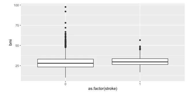
- Boxplot showing the BMI of individuals who experienced a stroke and those who didn’t
Average Glucose Level Comparison
Next, we compared the average glucose levels between the two groups. While the median levels were similar, there was a notable difference in variance between the groups, indicating a potential association between stroke and blood sugar levels.
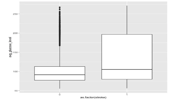
- Boxplot comparing the avg. glucose level between the two groups
Hypertension and Stroke
We analyzed the relationship between hypertension and stroke by creating a contingency table and conducting a chi-squared test. The results showed a significant association between having hypertension and experiencing a stroke.
| Yes(Hypertension) | No | |
|---|---|---|
| Yes(Stroke) | 66 | 183 |
| No | 432 | 4429 |
Table 1: Association between hypertension and stroke
Smoking Status and Stroke
Similarly, we assessed the relationship between smoking status and stroke using a contingency table and a chi-squared test. The test statistics revealed a statistically significant relationship between smoking and experiencing a stroke.
| No(Stroke) | Yes | |
|---|---|---|
| formerly smoked | 815 | 70 |
| Never smoked | 1802 | 90 |
| smokes | 747 | 42 |
| unknown | 1497 | 47 |
Table 2: Relationship between smoking status and having a stroke
Analysis and Evaluation
After conducting exploratory data analysis, we proceeded to build and evaluate predictive models.
Linear Regression
We trained a linear regression model and identified that age, hypertension, heart disease, and average glucose level were significant variables based on the p-values of the coefficients. The adjusted R-squared value indicated that only 7% of the outcome's variation was explained linearly by the covariates. Testing the model on the test dataset resulted in an accuracy of 0.83.
| oep. va riable: | stroke | R-squared: | 0.076 |
|---|---|---|---|
| Model: | OLS | Adj. R-squared : | 0.072 |
| Method: | Least Squares | F-statistic: | 20.08 |
| Da te : | Sun, 19 Har 2923 | Prob (F-statistic): | 3.07e-S6 |
| Time ' | 92:18:4& | Log-Likelihood | 99,626 |
| No. Observations:Of Residuals: | 3927 | AIC: | -199 |
| Of Mode\: Covariance Type: | 3916 | BIC: | -1852 . |
| coef | std err | t | P>|t | [0.025 | 0.975] | |
|---|---|---|---|---|---|---|
| const | -0.0929 | 0.019 | -4.769 | 0.000 | -0.131 | -0.055 |
| age | 0.0025 | 0.000 | 10.831 | 0.000 | 0.002 | 0.003 |
| hypertension | 0.0392 | 0.011 | 3.562 | 0.000 | 0.018 | 0.061 |
| heart_disease | 0.0464 | 0.015 | 3.140 | 0.002 | 0.017 | 0.075 |
| avg_glucose_level | 0.0004 | 7.16e-05 | 5.085 | 0.000 | 0.000 | 0.001 |
| bmi | -0.0006 | 0.000 | -1.348 | 0.178 | -0.001 | 0.000 |
| gender_ Male | 0.0017 | 0.006 | 0.277 | 0.782 | -0.010 | 0.014 |
| gender_Other | -0.0269 | 0.189 | -0.143 | 0.887 | -0.397 | 0.343 |
| ever_married_Yes | -0.0245 | 0.009 | -2.731 | 0.006 | -0.042 | -0.007 |
| work_type_Never_worked | 0.0290 | 0.045 | 0.648 | 0.517 | -0.059 | 0.117 |
| work_type_Private | 0.0099 | 0.009 | 1.073 | 0.283 | -0.008 | 0.028 |
| work_type_Self-employed | -0.0140 | 0.011 | -1.223 | 0.221 | -0.036 | 0.008 |
| work_type_children | 0.0528 | 0.016 | 3.352 | 0.001 | 0.022 | 0.084 |
| Residence_type_Urban | 0.0035 | 0.006 | 0.581 | 0.561 | -0.008 | 0.015 |
| smoking_status_formerly: smoked | 0.0072 | 0.010 | 0.711 | 0.477 | -0.013 | 0.027 |
| smoking_status_never smoked | 0.0019 | 0.008 | 0.224 | 0.823 | -0.014 | 0.018 |
| smoking_status_smoke | 0.0099 | 0.010 | 0.954 | 0.340 | -0.010 | 0.030 |
| Omnibus: | 3307.510 | Durbin-Watson: | 2.020 |
|---|---|---|---|
| Prob(Omnibus): | 0.000 | Jarque-Bera (JB): | 60531.132 |
| Skew: | 4.174 | Prob(JB): | 0.00 |
| Kurtosis: | 20.328 | Cond. No. | 7.85e+03 |
- Linear Regression Model in Python to Train the Dataset
Decision Tree
We utilized a decision tree model to predict stroke risk. After fitting the model on the test dataset, we achieved an accuracy of 0.91, which outperformed the linear regression model. The regression diagnostics are show by the plot
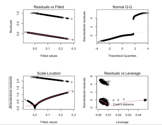
- Regression Diagnostics
Neural Network
A neural network model with two hidden layers and 64 cells was employed, and it was trained for 100 epochs. The model achieved a Mean Absolute Error (MAE) of 0.11 and an accuracy of 0.89, falling between the decision tree and linear regression models in terms of performance.
Appendix
import numpy as np
import os
import pandas as pd
from sklearn.model_selection import train_test_split
import statsmodels.api as sm
from sklearn.linear_model import LinearRegression
import tensorflow as tf
from tensorflow.keras.datasets import mnist
from tensorflow.keras.models import Sequential
from tensorflow.keras.layers import Conv2D, MaxPooling2D, Flatten, Dense
import tensorflow as tf
from tensorflow import keras
df=pd.read_csv("healthcare-dataset-stroke-data.csv")
df.columns
df=df.drop('id',axis=1)
df.columns
df=df.dropna()
X=df[['gender', 'age', 'hypertension', 'heart_disease', 'ever_married',
'work_type', 'Residence_type', 'avg_glucose_level', 'bmi',
'smoking_status']]
y=df['stroke']
lm = LinearRegression()
X_train = pd.get_dummies(data=X_train, drop_first=True)
X_test = pd.get_dummies(data=X_test, drop_first=True)
X_test['gender_Other']=[0]*982
new_order=['age', 'hypertension', 'heart_disease', 'avg_glucose_level', 'bmi',
'gender_Male', 'gender_Other', 'ever_married_Yes',
'work_type_Never_worked', 'work_type_Private',
'work_type_Self-employed', 'work_type_children', 'Residence_type_Urban',
'smoking_status_formerly smoked', 'smoking_status_never smoked',
'smoking_status_smokes']
X_test=X_test[new_order]
X_train1 = sm.add_constant(X_train) # add intercept term
model = sm.OLS(y_train, X_train1)
results = model.fit()
print(results.summary())
lm.fit(X_train, y_train)
lm.fit(X_train, y_train)
y1=lm.predict(X_test)
for i in range(982):
if y1[i]>.1:
y1[i]=1
else:
y1[i]=0
sum(m)/982
clf.fit(X_train, y_train)
y_pred = clf.predict(X_test)
accuracy = accuracy_score(y_test, y_pred)
mean = X_train.mean(axis=0)
std = X_train.std(axis=0)
X_train = (X_train - mean) / std
X_test = (X_test - mean) / std
model = keras.Sequential([
keras.layers.Dense(64, activation='relu', input_shape=(X_train.shape[1],)),
keras.layers.Dense(64, activation='relu'),
keras.layers.Dense(1)
])
model.compile(optimizer='adam', loss='mse', metrics=['mae'])
history = model.fit(X_train, y_train, epochs=100, validation_split=0.2)
test_loss, test_mae = model.evaluate(X_test, y_test)
print('Test MAE:', test_mae)