
Problem Description
This data analysis assignment using R revolves around various statistical questions and hypothesis-testing scenarios, covering diverse topics such as temperature, weight, heart rate, blood pressure, and drug effectiveness. Our objective is to employ statistical methodologies, including Z-tests, t-tests, confidence intervals, and bootstrapping, to derive conclusions and make data-driven inferences.
Question 1 - Investigating a Right Skewed Distribution of Values Using R
μ=98ºF
σ= 0.62ºF,
n = 35
Probability of Obtaining a Sample Mean of 98.2°F or Lower: We sought to determine the likelihood of obtaining a sample mean of 98.2°F or less by employing a Z-test.
P(X ̅≤98.2)=P((X ̅-μ)/(σ⁄√n)≤(98.2-μ)/(σ⁄√n))=P(Z≤(98.2-98)/(0.62⁄√35))
P(Z≤1.91)=.97193
The calculated probability was approximately 0.97193.
Result: The probability of obtaining a sample mean of 98.2°F or lower is estimated at 0.97193.
Probability of a Randomly Selected Individual with a Body Temperature of 98.2°F or Lower: In this part, we again applied the Z-test to ascertain the probability of an individual's body temperature being 98.2°F or lower.
P(X≤98.2)=P((X-μ)/σ≤(98.2-μ)/σ)=P(Z≤(98.2-98)/0.62)
P(Z≤0.32)=.62552
The result was roughly 0.62552.
Result: The probability of a randomly selected individual having a body temperature of 98.2°F or lower is 0.62552.
Probability of Obtaining a Sample Mean within 0.15°F of the Population Mean: We calculated the probability of achieving a sample mean within 0.15°F of the population mean using the Z-test.
Upper of X ̅=98+0.15=98.15
Lower of X ̅=98-0.15=97.85
P(97.85
= (Z<(98.15-98)/(0.62/√35))-P(Z<(97.85-μ)/(0.62/√35))
P(-1.43
=0.84728
The result was approximately 0.8473.
Result: The probability of obtaining a sample mean within 0.15°F of the population mean is estimated at 0.8473.
Probability of Obtaining a Sample Mean Differing by More than 0.2°F: This segment focuses on the probability of obtaining a sample mean differing from the population mean by more than 0.2°F.
X ̅=98+0.2=98.2 ºF
P(X>98.2)=1-P((X ̅-μ)/(σ/√n)<(98.2-μ)/(σ/√n))=1-P(Z≤(98.2-98)/(0.62/√35))
P(Z>1.91=1-.97193
=0.02807
The calculated probability was about 0.0281.
Result: The probability of obtaining a sample mean that differs from the population mean by more than 0.2°F is approximately 0.0281.
Question 2
2.1. Confidence Interval for Population Mean: We computed a 95% confidence interval for the population mean, resulting in the interval (7.7135, 11.6865).
CI=X ̅± Z×σ/√n
Z=1-0.05/2=0.975
The z-score 0.975 is 1.96
CI=9.7± 1.96×4.3/√18
(7.7135, 11.6865)
Result: We are 95% confident that the actual population mean for all male postal workers of the acceptable load is within the interval (7.7135, 11.6865).
2.2. Effect of Sample Size and Confidence Level on Confidence Interval: In this part, we discussed how increasing the sample size narrows the confidence interval, while increasing the confidence level widens it.
2.3. Hypothesis Test: A hypothesis test was performed to ascertain whether the population mean differs from 12kg. The null hypothesis was rejected based on the calculated test statistic.
Result: There is compelling evidence to suggest that the population mean acceptable load for all male postal workers is different from 12kg at the 5% significance level.
Question 5
In this question, we discussed Type I and Type II errors in the context of two hypotheses related to symptoms and their causes. A hypothesis test was conducted to determine if the mean heart rate after 15 minutes of Wii Bowling is different from the known mean heart rate after 6 minutes of walking on the treadmill, and a conclusion was provided.
Module 06 Questions
Question 6 - Hypothesis Test with Sample Size and Power Analysis:
X ̅=101 bpm
s= 15 bpm,
n = 14
μ=98 bpm
6.1. Hypothesis Test (t-test): A hypothesis test was performed to determine if the mean heart rate after 15 minutes of Wii Bowling differs from 98 bpm. The null hypothesis was not rejected.
Result: There is insufficient evidence to support the claim that the mean heart rate after 15 minutes of Wii Bowling is different from 98 bpm at the 1% significance level.
6.2. Hypothesis Test for a Higher Mean Heart Rate: Another hypothesis test was conducted to determine if the mean heart rate after 15 minutes of Wii Bowling is higher than 66 bpm. The null hypothesis was rejected.
Result: There is substantial evidence to support the claim that the mean heart rate after 15 minutes of Wii Bowling is higher than 66 bpm at the 1% significance level.
Question 7 - Confidence Interval and Hypothesis Test for Blood Pressure:
X ̅=140mmHg
σ= 25mmHg
n = 61
μ=
CI=[134.651, 145.349].
The level of confidence did they use
Margin of error (E)=(UCL-LCL)/2
=(145.349-134.6511)/2
=5.34895
E=Z×σ/√n
5.34895=Z×25/√61
Z=1.671
Z_1.671=.95254
≈0.95
=95%
The level of confidence used is 95%
The true mean for SPS among people with glaucoma is lie between 134.651 and 145.349 intervals.
We are 95% confident that the true mean SBP among people with glaucoma is within 134.651 and 145.349 intervals.
Test the null hypothesis H0: Mean SBP for people with glaucoma is 144
The significance level of the hypothesis test that corresponds to this confidence interval is 5%
Since the mean of 144 of glaucoma is within the interval, we fail to reject the null hypothesis. Thus, there is no sufficient evidence to support the claim that the mean SBP for people with glaucoma is different from 144 at the 5% significance
Result: The confidence interval suggests that we are 95% confident the true mean SBP among people with glaucoma is within the interval (134.651, 145.349). The hypothesis test did not provide sufficient evidence to support the claim that the mean SBP for people with glaucoma is different from 144 mmHg at the 5% significance level.
Question 8 - Drug Effectiveness and Type II Error:
In this question, we formulated the null and alternative hypotheses for a drug's effectiveness and calculated the probability of committing a Type II error.
X ̅=1.3 hours
σ= 0.25 hours
n = 36
μ=1.5 hours
The null and alternative hypotheses
H_0=1.5 hours
H_1≠1.5 hours
The parameter interest is the brand name drug is known to relieve symptoms at 1.5 hours, on average, after administration of the drug.
The probability that they committed a Type II error
P(X=1.5)= (Z=(1.3-μ)/(σ/√n))
= (Z<(1.3-1.5)/(0.25/√36))
P(Z=-4.8)=0.0000
The probability that they committed a Type II error is 0.0000
The probability that the null hypothesis will be rejected
P(X=1.5)= (Z=(1.3-μ)/(σ/√n))
= (Z<(1.4-1.5)/(0.25/√36))
P(Z=-2.4)=.00734
The probability that the null hypothesis will be rejected is 0.000734
A sample would the researchers need if they wanted their test to have at least 87% power to detect a 15 minute reduction in mean time to cessation when using the generic drug compared to using the brand name drug
E=0.25
0.87 from z table is given as 1.12
E=Z×σ/√n
0.25=1.12× 0.25/√n
n=1
The researchers need if they wanted their test to have at least 87% power to detect a 15 minute reduction in mean time to cessation when using the generic drug compared to using the brand name drug 1
Question 3 - Data Distribution and Bootstrapping:
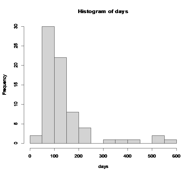
Fig 1: Histogram of survival time skewed to the right
The histogram of days of survival was analyzed, indicating a right-skewed distribution. Bootstrapping was used to determine if the sampling distribution of the sample mean is approximately normal for both a large and a small sample.
Use bootstrapping with B = 1000 bootstrap samples to either confirm or deny that the sampling distribution of the sample mean based on 72 survival times is approximately normal.
>boot::boot(data = days, statistic = cor, R=1000)
ORDINARY NONPARAMETRIC BOOTSTRAP
Call:
boot::boot(data = days, statistic = cor, R = 1000)
Bootstrap Statistics :
original bias std. error
t1* 0.7635205 -0.7656686 0.1215847
The standard error from the bootstrap is 0.1215847. Based on the bootstrap standard deviation of the mean, there is low variations in the survival times. Hence, the distribution is normally distributed.
The CLT says that the standard error of the sample mean is given by σ/√n.
σ=√(var(x))
σ=√11926.5256359
=109.2086334
SE =109.2086334/√72
=12.87036
The bootstrap standard error of the mean computed in part (b) is not to the standard error based on the CLT.
The bootstrap distribution suggest that the sampling distribution for the sample mean based on 20 survival times is closer to normal or farther from normal than the sampling distribution of the sample mean based on 72 survival times
>boot::boot(data = days1, statistic = cor, R=1000)
ORDINARY NONPARAMETRIC BOOTSTRAP
Call:
boot::boot(data = days1, statistic = cor, R = 1000)
Bootstrap Statistics :
original bias std. error
t1* -0.2044124 0.2010833 0.2290329
The standard error from the bootstrap based on 20 survival is 0.1215847
The sample mean based on 20 survival times is further from the normal than the sampling distribution of the sample mean based on the survival times.
Result: The bootstrap standard error for the large sample suggests that the distribution is normally distributed, while the small sample exhibits a larger bootstrap standard error, indicating a departure from a normal distribution due to the smaller sample size.