
Problem Description
The data analysis assignment aimed to predict the age of abalones, marine snails also known as ear shells or sea ears, from their physical measurements. Traditional methods of determining abalone age involve a time-consuming process of cutting the shell, staining it and counting the rings under a microscope. In this exercise, we sought to develop a method for predicting abalone age using easily obtainable physical measurements. The central question was whether it is possible to predict the age of an abalone based on these measurements.
Data Source: For this assignment, we utilized the "Abalone Data Set" available in the UCI Machine Learning repository. The dataset contains 4,177 observations, each with 9 attributes:
- Sex: Nominal, with values M (Male), F (Female), and I (Infant).
- Length: Continuous measurement in millimeters, representing the longest shell measurement.
- Diameter: Continuous measurement in millimeters, perpendicular to the length.
- Height: Continuous measurement in millimeters, with meat in the shell.
- Whole weight: Continuous measurement in grams, indicating the weight of the whole abalone.
- Shucked weight: Continuous measurement in grams, representing the weight of the meat.
- Viscera weight: Continuous measurement in grams, indicating the gut weight (after bleeding).
- Shell weight: Continuous measurement in grams, after being dried.
- Rings: An integer value, and the age in years can be calculated by adding 1.5 to this value.
The primary objective was to predict the "Rings" variable based on the other measurements, given that "Rings" is challenging to obtain directly.
Data Analysis Methods: We employed a multiple linear regression approach to address the question. While the "Rings" variable takes integer values, the fact that these integers range from 1 to 29, with a natural order, allowed us to treat it as a continuous variable. This led us to use a regression setup with 8 predictor variables.
The dataset was randomly split into a training set (75% of the data) and a test set. We measured model performance using the mean squared error on the test data.
Model Development:
1. Initial Model: The initial multiple linear regression model considered all predictors. The estimated regression equation was:
Rings ̂ = 3.59 - 0.875 × I(Sex = I) - 0.008 × I(Sex = M) - 0.721 × Length + 9.505 × Diameter + 22.145 × Height + 9.266 × WholeWeight - 20.215 × ShuckedWeight - 10.945 × VisceraWeight + 6.642 × ShellWeight
- In this model, all predictors except "Length" and the indicator for male sex were significant at the 0.01 level. The mean squared error on the test data was 5.365.
- Refined Model: To simplify the model, "Length" was removed from the regression, and the indicator for male sex was omitted, merging the two genders (M and F) into a single category. The refined regression equation was:
Rings ̂ = 3.547 - 0.873 × I(Sex = I) + 8.722 × Diameter + 22.103 × Height + 9.266 × WholeWeight - 20.244 × ShuckedWeight - 10.976 × VisceraWeight + 6.662 × ShellWeight
1. The adjusted R-squared value and coefficients did not change significantly. The mean squared error on the test data was 5.373.
Findings: The two regression models provided reasonably good, but not highly accurate, predictions of abalone age based on physical measurements. The root mean squared error for both models was approximately 2.32. However, graphical analysis revealed that the residuals may not be normally distributed, suggesting that a transformation on the y-variable could be beneficial. Despite their limitations, these regression models offer some utility in predicting abalone age using readily available physical measurements.
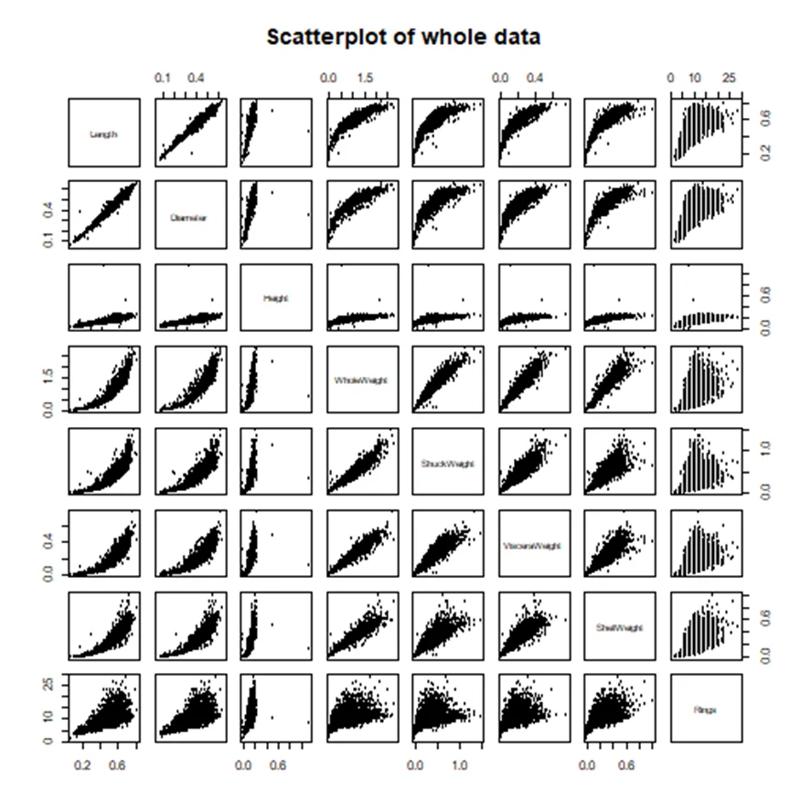
Fig 1: Scatterplot of the Whole Data
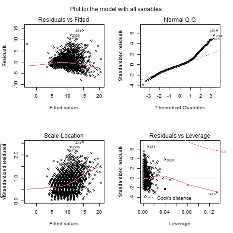
Fig 2: Plot for the model with all the variables
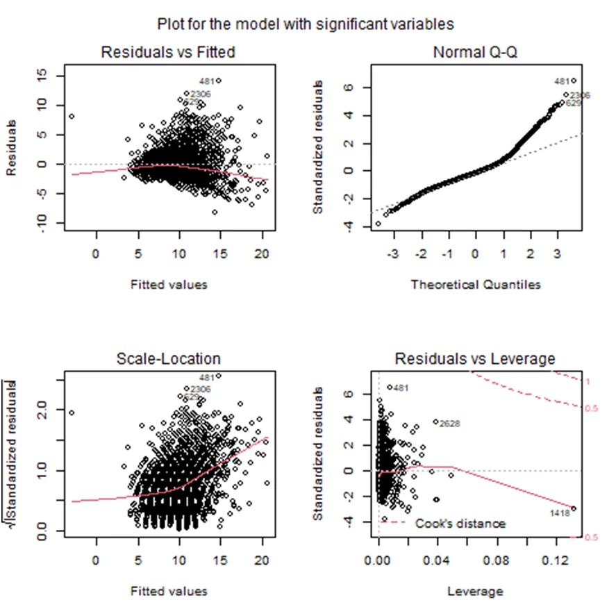
Fig 3: Plot for the model with significant variables
TABLES
Table 1: (Summary statistics)
| Sex | Length | Diameter | Height | |
|---|---|---|---|---|
| Min. | Min. | :0.0000 Min. | ||
| Length:4177 | :0.075 | :0.0550 | ||
| Class :character | 1st Ou. | :0.450 | 1st Qu.:0.3500 | Qu.:0.1150 1st |
| Mode :character | Median | :0.545 | Median :0.4250 | :0.1400 Median |
| Mean | :0.524 | :0.4079 Mean | :0.1395 Mean | |
| 3rd | Qu.:0.615 | 3rd Qu.:0.4800 | 3rd Qu. .:0.1650 |
| Whole | Weight | Shuck | Weight | Viscera | Weight | Shell | Weight |
|---|---|---|---|---|---|---|---|
| Min. | :0.0020 | Min. | :0.0010 | Min. | :0.0005 | Min. | :0.0015 |
| 1st | Qu. :0.4415 | 1st | Qu.:0.1860 | 1st Qu. :0.0935 | 1st | Ou :0.1300 | |
| Median :0.7995 | Median | :0.3360 | Median :0.1710 | Median | :0.2340 | ||
| Mean | :0.8287 | Mean | :0.3594 | Mean | :0.1806 | Mean | :0.2388 |
| 3rd Qu. :1.1530 | 3rd | Qu. :0.5020 | 3rd Qu. :0.2530 | 3rd Qu :0.3290 | |||
| Max. | :2.8255 | Max. | :1.4880 | Max. :0.7600 | Max. | :1.0050 |
Rings
Min. : 1.000
1st Qu.: 8.000
Median: 9.000
Mean: 9.934
3rd Qu.:11.000
Max. :29.000