Mastering OLS Regression Models and Stata: In-Depth Analysis and Interpretation

Problem Description

Explore the intricacies of OLS regression models and their real-world applications in Stata assignment. Delve into the impact of omitted variable bias, the estimation of coefficients, and the effect of covariates on regression outcomes. Transition to regression modeling questions, interpreting results, and understanding the implications of omitted variables. This comprehensive exploration encompasses the mathematical and practical aspects of regression analysis.

Question 1.1: The Impact of Omitted Variables on OLS Regression Models

In this question, we delve into the concept of omitted variable bias and its influence on Ordinary Least Squares (OLS) regression models. The key issue is that when a crucial variable, Z, is omitted from the model, it can lead to bias in the estimated coefficient β₁. This bias occurs because Z is correlated with both the independent variable X and the dependent variable Y. As a result, β₁ not only captures the relationship between X and Y but also the indirect relationship between Z and Y through X.

Question 1.2: Estimating β₁ in the Presence of Omitted Variables

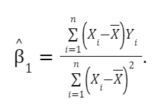
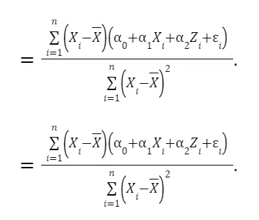
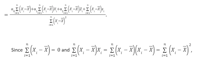
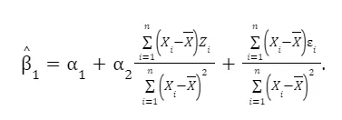
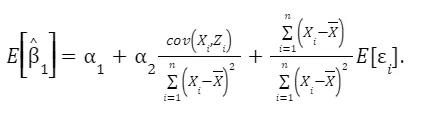
This focuses on the process of estimating the coefficient β₁ while taking into account the presence of omitted variables like Z. We derive the formula for estimating β₁ and explore its components in detail. This includes breaking down how Z and ε influence the estimation. By manipulating the formula, we understand that β₁ equals α₁ plus an additional term involving Z and ε. This step helps to see how omitted variables can impact the accuracy of β₁.

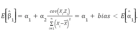
Taking expectations, we have

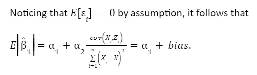
Finally, we can see that the 1 captures the true relationship between only if cov(Xi,Zi)=0, which is NOT the case.

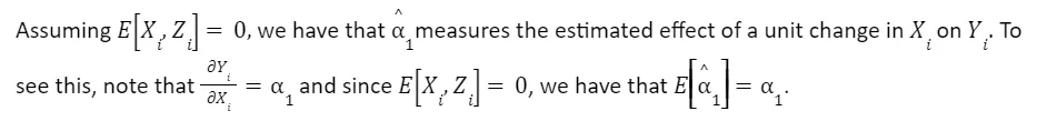
Question 1.3: Estimating the Effect of X on Y When ε is Conditioned on X and Z

This question extends our understanding of how X affects Y, assuming that ε is conditioned on both X and Z. We establish that α₁ measures the estimated effect of a one-unit change in X on Y. The assumption here is that ε is orthogonal to X and Z. This allows us to interpret α₁ as the causal relationship between X and Y while controlling for the influence of Z.

Question 1.4

Questions 1.4 delve into OLS residuals and their connection to Z. Part 'a' clarifies that rᵢ represents the OLS residual of observation i, which captures the portion of Xᵢ that is not correlated with Zᵢ. Part 'b' introduces α̂₁, the estimated coefficient when Y is regressed on rᵢ, essentially isolating the part of X that is unrelated to Z. It provides an intuitive explanation of how α̂₁ estimates the effect of X on Y while controlling for Z. Part 'c' delves into the implications of the first-order conditions from the OLS minimization problem.

Question 1.4-a

r ̂i is the OLS residual of observation i from the simple regression of Xi on Yi. Specifically, the residuals r ̂i are the part of Xi that is NOT correlated with Zi.

Question 1.4-b

X1 is the estimated 1 of the modelSince ri measures only the variation of X that is uncorrelated with Z, then indeed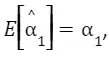the true relationship between X and Y. We can say intuitively that it estimates the effect of X on Y partialling out the effect of Z.

Question 1.4-c

The first order conditions from the OLS minimization problem imply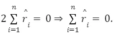Then,

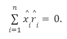
Question 1.5, 1.6, 1.7: Impact of Covariates and External Validity

Questions 1.5 through 1.7 examine how the presence of covariates impacts the relationship between X and Y. Part '1.5' explores a scenario where the number of younger workers (Xᵢ) affects both the number of bars and unprotected sexual relationships, leading to a higher number of children born. This leads to a positive covariation between Xᵢ and Yᵢ.

In part '1.6,' we discuss how the presence of covariates, such as Zᵢ and the correlation of Xᵢ and Yᵢ with Zᵢ, can influence the estimate of β₁ and introduce bias. Part '1.7' extends this discussion by considering a different covariate, education levels (Zᵢ), and its potential effects on Yᵢ. This raises questions about the impact of these covariates on the relationship between X and Y and their implications for external validity.

Question 1.5

A state with more younger workers have more bars, in equilibrium, in face of a higher consumption of alcohol. This may translate in a higher number of unprotected sexual relationships in the month of January due to the effect of alcohol on people, thus resulting in a higher number of children born in the state during September. In this case,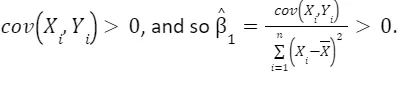

Question 1.6

Letbecause we expect that states with higher number young workers present a higher number of bars. Also,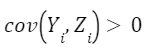because we expect that a higher number of young workers to be positively correlated with more children born, given that older people have less kids and very young people do not have kids (for obvious reasons), so x2>0. Adding the argument in the previous question, we have thatThen,

Question 1.7

LetWe expect that a state with more educated population, and thus more educated women, have a lower birth rate because the opportunity cost of having children is higher, soAdditionally, we expect a more educated state to have higher income and, as a result, a higher number of bars, which impliesSincewe have that

Question 2: Transition to Regression Modeling

We now transition to a set of questions that revolve around regression modeling. Each of these questions will focus on applying regression techniques to real-world data and interpreting the results.

Question 2-1: Estimating Equation (1) and Reporting Results

In this question, we will estimate the relationship between variables as described in equation (1) and provide a detailed report of the results. We will interpret the coefficients and explore the implications of this regression.

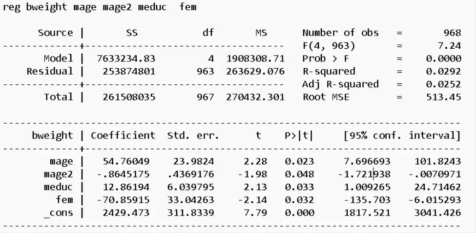
Fig 1: Estimated Results of equation 1

Question 2-2: Interpreting β₃ and Its Practical Significance

Here, we will analyze the meaning of the coefficient β₃ in the context of the regression model. We will explain the practical significance of β₃ and provide a clear interpretation of how changes in the independent variable, expressed in years of education, impact the dependent variable (weight at birth).

Question 2-3: The Interpretation of β₀ and Its Real-World Significance

In this question, we will dive into the interpretation of the coefficient β₀, the intercept, and its practical implications. We will discuss the significance of β₀ in a real-world context, considering the limitations and assumptions involved.

Question 2-4, 2-5: Generalized Expression and Turning Points

Questions 2-4 and 2-5 are interrelated. In 2-4, we will derive a generalized expression for the derivative of birth weight with respect to maternal age. In 2-5, we will determine the point at which predicted birth weight begins to decrease concerning maternal age. These questions will involve mathematical and practical analysis of the regression results.

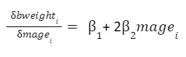
Question 2-4: What is the generalized expression for d bweight/d mage from equation (1)?

Taking the equation we are estimating:

And derivating w.r.t. mage_i, we have:

Question 2-5: At what point does predicted birthweight begin to decrease with respect to maternal age?

Using the results we obtained in q 2-4 and q 2-1, we have

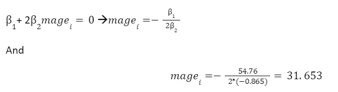
Hence, after half of the 31st year of age the predicted birth decreases with age.

Question 2-6, 2-7: Explaining Regression Results in Non-Technical Terms

In these questions, we will explain the implications of the regression results in a way that is understandable to a non-technical audience. We will also consider the assumptions and validity of the results and analyze their applicability to different contexts, such as the United States in 2022 and Kenya in the 1990s.

Question 2-6: Assume this model is internally valid and it perfectly captures the determinants of birthweight and that birthweight is a good predictor of future health, explain, in a way that your non-Econ, non-mathematical friend would understand, what the result in question (5) means.

Under the assumption of internal validity, my explanation will be the following one:

My result in question 5 means that age of the mother has a positive impact on the health of a child. Nevertheless, this positive impact tends to decrease after a certain age. Hence, the health of a kid (ceteris paribus) peaks at a certain age of the mother, around 31 years old. Before that age, it increases with age of the mother. After that age, it decreases with the age of the mother.

Question 2-7: Given the assumptions of internal validity provided in question (6) and the fact that this data accurately represents all U.S. born children in 1993 (a very large sample!) can we make a statement about the impact of an additional year of maternal educational attainment on birthweight in the United States in 2022? Why or why not? What about a statement on this relationship in Kenya in the 1990s? Why or why not? Be specific about your reasoning and try to make a convincing argument.

Under the assumption of internal validity and of representativeness of the sample of children born in the US in 1993, I believe we can claim the results on the impact of educational attainment of mother on child’s health, tend to keep external validity with respect to a sample of children born in 2022. This because returns of education driving the benefits on child’s health have probably not dramatically changed in the last 30 years in the US, hence external validity is likely to be preserved.

Contrarily, it is likely that returns of education were extremely different (and in particular, extremely lower) in 1990s Kenya than in 1993s US. This implies that the mechanisms driving the result we observed are probably not in place in this different setting. An example of a potential mechanism could be that more educated mothers earn higher salaries, and hence have access to better food and medicines during the pregnancy. If returns of education are lower, than this positive mechanism is missing.

Question 2-8: Addressing Biases and Limitations in the Regression

In this question, we will discuss potential biases and limitations in the regression analysis, particularly the omission of critical variables. We will provide an intuitive argument for why the regression might not fully explain the impact of maternal age on lower birth weight within the sample.

Removing the assumptions we made in question (6), what is an intuitive argument for why this regression may not be able to tell us much about how maternal age impacts lower birthweight within our sample?

In this analysis several potential biases can arise, in particular in terms of omitted variable. An example that can easily come to mind is wage. We can expect it to be correlated with the age of the mother (in a classic life-cycle model fashion) and with the health of the child, since as we mentioned before higher wages mean better provision of goods during the pregnancy.

Hence, weight at birth could be correlated positively with mother’s age just because the mother is in a better position in her life-earnings cycle.

More generally, it is well known that in wealthier and more educated families women tend to have children at higher ages, hence once again the driver of the better conditions of the child might be driven simply by the better economic condition of the mother or of the family.

Question 2-9: Analyzing the Impact of Omitting Variables on ψ₁

This question will explore the effects of omitting variables on ψ₁ and compare it to γ₁ and γ₂. We will discuss how the omission of variables can lead to differences in the estimated coefficients and their implications for the model.

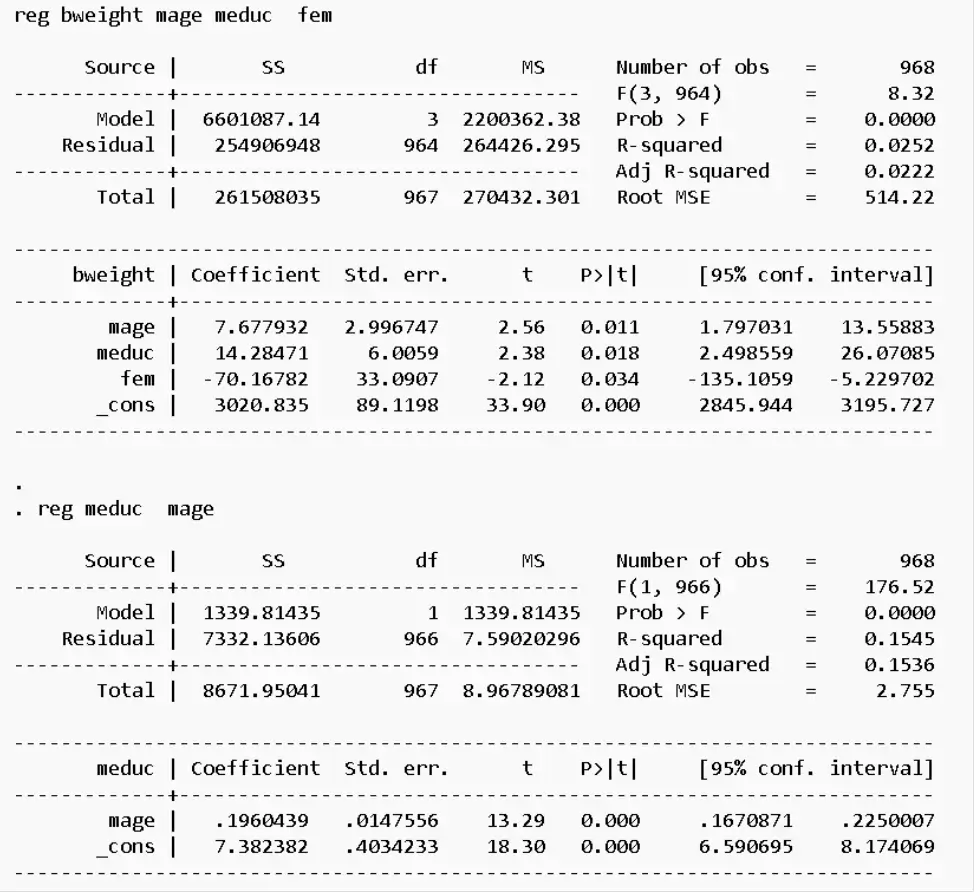
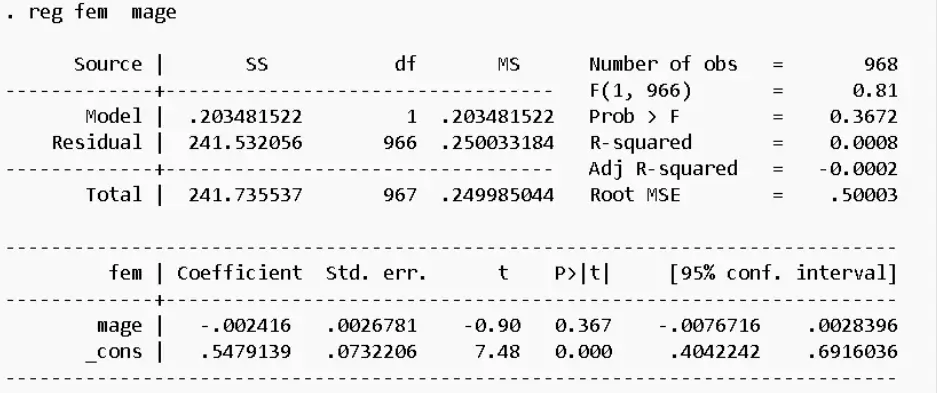
Fig 2: Impact of Omitting Variables on ψ₁

In equation 5, we would be estimating the equation leaving out the variable meduc. This implies that the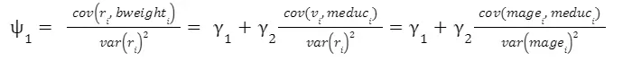

In our case γ_2 is positive and so is the correlation between meduc and mage. Hence,

Question 3: A Shift to a New Set of Questions on Regression Analysis

Transitioning to a new set of questions related to regression analysis, we will explore various aspects of regression modeling and interpretation.

Question 3-1: Regressing Award on Age of Death

This question will involve regressing the variable 'award' on 'age of death.' We will report and interpret the results, specifically looking at the slope and intercept and their implications for understanding the relationship between these variables.

When we regress award on age of death, we have a slope of -1.18 and a constant of 141.98. This implies that for each additional year of age of the decedent the award decreases of 1180$. The intercept represents the (expected) award if the age of the decedent is the minimum in the sample and would be 141977$.

Question 3-2: Understanding Variance, SST, and ESS

In this question, we will delve into the concepts of variance, Sum of Squares Total (SST), and Explained Sum of Squares (ESS). We will explore their relationships and discuss their significance in the context of regression analysis.

The variance of awards is 4240.98027. In our regression, the SST is 631906.06. The two are related since the SST is given by the variance of the output multiplied by the number of degrees of freedom (number of observations – 1). The ESS is the portion of the SST explained by the model. In this case, it is equal to 33551.678.

Question 3-3: Calculating R² and Interpreting its Significance

This question focuses on calculating and interpreting the coefficient of determination, R². We will discuss how R² measures the proportion of variance explained by the model and its practical significance.

The R^2 will be ESS/SST = 33551.678/631906.06 = 0.05309599. This is the same result we obtain from the STATA output (0.0531).

Question 3-4: The Impact of Taking Logarithms on Variable Distributions

In this question, we explore the effect of taking logarithms of variables on their distributions. We will analyze how this transformation can impact the normality assumption and the interpretability of the regression model.

Fig 3: Impact of Taking Logarithms on Variable Distributions

From the first row of the graph, it can be observed that the distribution “award” variable is clearly left skewed with some outliers between 300 and 400. After taking log, the variable becomes slightly right skewed, but way more similar than a normal distribution. Regarding the second row, we can see that the distribution of the variable “age” is also somewhat skewed with an outliers around 100. After taking logs, the distribution of the transformed variable also becomes more close to a normal. Therefore, the first advantage of taking logs is to make the normality assumption more likely to hold.

Additionally, the interpretation of a log-log regression can be more easily understood because (though not exclusively) logs are unit free.

Question 3-5: Comparing Models and Their R² Values

This question involves comparing different regression models and interpreting their R² values. We will discuss why one model might be considered better than another, considering the increase in explanatory power and the implications for understanding the relationship between variables.

It is true that a log-log model may be easier to interpret. Nevertheless, it is merely a transformation of the original variables and an increase in the R² does probably reflects this change in scale. Specifically, the log-log regression displays a higher R² because the observations of the dependent variable become more “centered” around its (new) median, thus naturally making the independent variable to have a higher explanatory power in terms of variability.

Question 3-6: Analyzing the Impact of Additional Variables on Explanatory Power

In this question, we will examine the impact of including additional variables in the regression model. We will compare models to understand how the inclusion of squared log(age) affects the explanatory power of the model and its implications for understanding the relationship between variables.

While the estimation of model (7) yields an R² = 0.0770, the estimation of model (8) yields a higher value of R² = 0.1159. In words, in the first case the explanatory variable can account for about 7.7% of the variability in the explained variable, while in the second case the independent variables account together for about 11,59% of the variability in the dependent variable. This result is expected because the inclusion of more variables cannot reduce the value of the R². Even though the result is expected, the increase in the explanatory power seems to be relevant with the inclusion of the squared log(age).

For model (7),

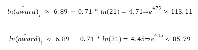
For model (8),

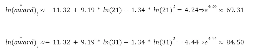
I believe that the best model to calculate the award is the (8) because it allows for non-linearities.