
Problem Description
The Econometric Analysis assignment at hand delves into the analysis of consumption expenditures and their relationship with income, exploring the influence of other variables such as housing prices, consumer sentiment, and economic recessions. The primary aim is to understand the dynamics of consumption, investigating its correlation with various factors and the implications this has for economic modeling.
Model and Theoretical Foundation
The foundation of this analysis lies in economic theories, primarily originating from the work of John Maynard Keynes. Keynes proposed that consumption increases with income but at a rate less than proportionate, giving rise to the concept of the marginal propensity to consume (MPC). Subsequent economists, including Milton Friedman and Modigliani-Brumberg, introduced various interpretations of income's role in consumption decisions.
Econometric Model: The consumption model is expressed as,
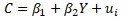
Here, C represents consumption, Y denotes income, and ul is the error term. The parameters β_1 and β_2 represent autonomous consumption and the marginal propensity to consume, respectively. The model can be extended to include control variables such as housing prices and consumer sentiment to better explain consumption patterns i.e.,
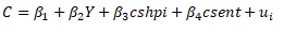
Where cshpi represents US home price index while csent is the consumer sentiment index. Furthermore, the impact of economic recessions on consumption is considered as follows:

Where increc is the interaction of Y and a dummy variable which equals 1 when there is recession and 0 otherwise.
Data Source and Variables: Data was sourced from the Federal Reserve Bank of St. Louis. Key variables include:
- C: US real personal consumption expenditures (Billions of chained 2012 dollars)
- Y: US real disposable personal income (Billions of chained 2012 dollars)
- cshpi: Seasonally adjusted S&P/Case-Shiller US Home Price Index (Index)
- csent: University of Michigan Consumer Sentiment Index (Index)
- increc: A dummy variable representing whether the US is in a recession (1 for recession, 0 otherwise)
Results: The analysis yielded results across three models:
Model 1:
- MPC: 0.694 (If income increases by $1, consumption increases by $0.69)
- Autonomous consumption: $2,517.98
Model 2 (With Housing Prices and Consumer Sentiment):
- MPC: 0.595
- Autonomous consumption: $2,315.13
- Housing price index positively impacts consumption
- Consumer sentiment index positively impacts consumption
Model 3 (Including Recession Interaction):
- MPC is greater when there is no recession (0.59) compared to during a recession (0.57)
All models exhibited high R-squared values (0.901 to 0.914), indicating that independent variables explain 90.1% to 91.4% of consumption variation. F-tests for model significance returned p-values below 0.001, confirming the joint significance of independent variables.
Diagnostic Test for Model 3:
- Autocorrelation: Rejected null hypothesis (model suffers from autocorrelation)
- Heteroscedasticity: Rejected null hypothesis (model suffers from heteroscedasticity)
- Omitted variable bias: Rejected null hypothesis (model suffers from omitted variable bias)
- No evidence of multicollinearity
The autocorrelation test showed that the null hypothesis of no autocorrelation is rejected (χ^2=135.12,p<.001) which implies that the model suffers from autocorrelation. The heteroscedasticity test showed that the null hypothesis of no heteroscedasticity is rejected (χ^2=270.03,p<.001) which implies that the model suffers from heteroscedasticity. The Ramsey RESET test for omitted variable bias showed that the null hypothesis of no omitted variable is rejected (F=113.81,p<.001) which implies that the model suffers from omitted variable bias.
| Test | Statistics(p) |
|---|---|
| Breusch-Godfrey LM test for autocorrelation | 135.12(<.001) |
| heteroscedasticity | 270.03 (<.001) |
| Omitted variable test | 113.81 (<.001) |
Table 1: Diagnostic test result
The variance inflation factor test is used to test for multicollinearity. The result present evidence of no multicollinearity as none of the variables have VIF greater than 10.
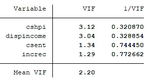
Table 2: Test for Multicollinearity
A histogram of residuals indicates a violation of the normality assumption.
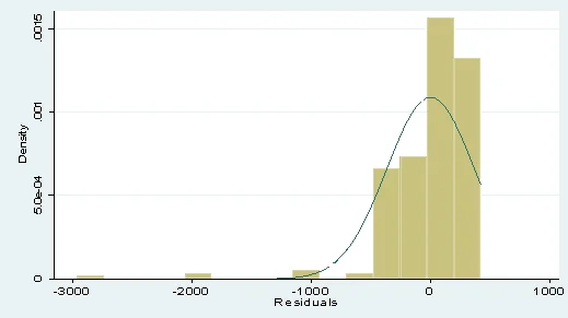
Fig 1: Histogram to test for normality of residuals
Analysis and Suggestions: The results support established economic theories regarding income-consumption relationships. However, the models display violations of key linear regression assumptions, casting doubt on their correctness. To improve the model, it is suggested to include lags of consumption to address autocorrelation and robust standard errors to tackle heteroscedasticity. These adjustments can enhance the model's accuracy and validity.
This assignment provides valuable insights into the intricacies of consumption expenditure modeling, showing the practical application of economic theories in real-world scenarios while highlighting the importance of model diagnostics and improvements.