
Problem Description:
Addressing housing market dynamics and financial strategies, this Statistical Analysis assignment explores factors influencing housing prices, evaluates residential firm valuation and risk, and offers policy advice. It also covers options trading strategies, portfolio hedging with futures, option pricing via Monte Carlo simulations, and the relationship between implied volatility curves. Finally, it discusses potential arbitrage opportunities in the stock market.
Section A
1) Housing Market Analysis
Problem: Analyze the factors influencing housing prices in the past decade.
Solution:
Over the last decade, the global housing market has experienced unexpected strength during the COVID-19 pandemic. Prices have risen in many middle- and high-income countries. This pattern is attributed to three key factors: monetary policy, fiscal policy, and changing consumer preferences. Central banks worldwide lowered policy rates, reducing mortgage borrowing costs. Governments provided fiscal support to households, protecting incomes and preventing foreclosures. As remote work became more prevalent, the demand for larger and better-quality homes increased. While the housing market has not been the cause of economic problems this time, its long-term performance remains uncertain.
2) Valuation and Risk of Residential Firms
Problem: Assess the valuation and risk associated with residential firms' stocks.
Solution:
In the current economic environment, residential firms face risks, such as a potential housing market downturn, changes in government policies, and economic uncertainty due to COVID-19. However, these firms may experience potential returns due to the low-interest rate environment and growth in the housing market. The risk of residential firms' stocks is moderately high due to anticipated price declines and rising interest rates, making mortgage qualification more challenging.
3) Advising the Secretary of the Treasury
Problem: Advise Secretary Mnuchin on supporting the housing market post-COVID.
Solution:
It's crucial for the government to support the housing market during the pandemic-induced economic downturn. However, the approach should strike a balance. Simply intervening by lowering taxes, providing subsidies, and loosening mortgage standards may offer short-term support but lead to long-term instability through mispriced houses. Allowing the market to equilibrate on its own could lead to sharp price declines and worsen the recession. Therefore, targeted support, such as suspending foreclosures and offering mortgage repayment assistance, would be a more controlled and sustainable approach.
Section B
1) Butterfly Spread
Problem: Consider the butterfly spread in which you buy a call with strike $80, buy a call with strike $90, and sell two calls with strike $85. The calls are European and expire in 6 months. The underlying stock has current price $83.
(a) Draw the payoff diagram of the spread. What is the largest possible payoff?
(b) Suppose the $80 strike call costs $8 and the $90 strike call costs $5. What is the most the $85 strike call can cost to preclude arbitrage? Explain.
(c) Say the $85 strike call costs $7. Show there is an arbitrage and calculate the guaranteed minimum profit.
Solution
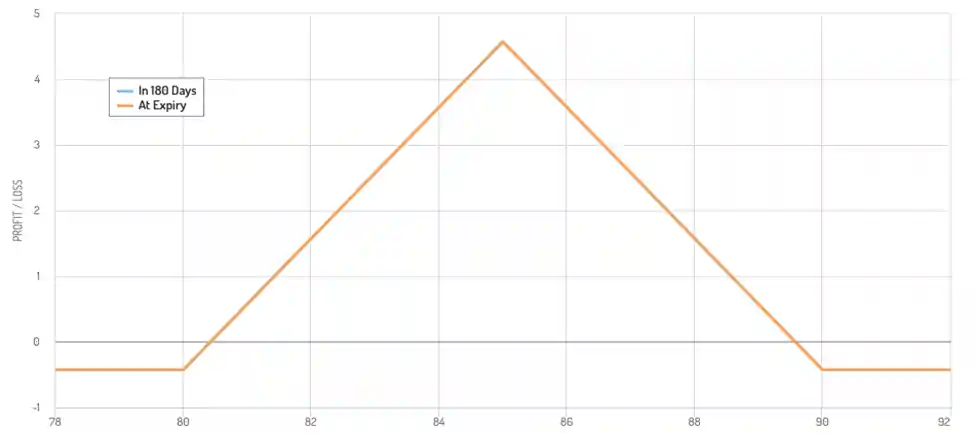
Fig 1: payoff diagram of the spread
(a) The largest possible payoff occurs when the stock price is at $85.
(b) To preclude arbitrage, the $85 strike call cost must be less than the net premium paid for the $80 and $90 strike calls, which is $13. Therefore, the $85 strike call must cost $6.5 or less.
(c) If the $85 strike call costs $7, arbitrage is possible, and the minimum profit is $1.
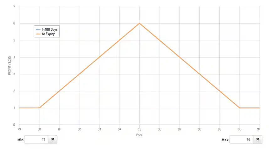
Fig 2: Payoff diagram showing there is an arbitrage and calculate the guaranteed minimum profit.
2) Asset-or-Nothing Options
Problem: An asset-or-nothing option provides a payoff equal to the asset price if the asset price is above the strike price and zero otherwise. Suppose the asset currently sells for $20 and has volatility 30%. The risk-free rate is 5%.
(a) Use a two-step tree to compute the price of a 2-month asset-or-nothing put option on the asset with strike $22.
Solution:

Fig 3: 2-step tree diagram
- The option price is $2.259
(b) Use your tree to compute the price of a 2-month European call option with strike $22.
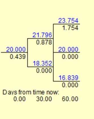
Fig 4: 2-step tree diagram
The option price is $0.439
(d) Which option price is larger? Sketch their payoff diagrams to show this is not by accident.
- The put option is larger because it is currently in the money
(e) BONUS: Show that it is always optimal to early exercise an American asset-ornothing option on a stock.
- t is generally not optimal to early exercise an American asset-or-nothing option on a stock. This is because exercising the option early means forfeiting any potential future gains from the stock. If the stock price is expected to rise, the option holder can simply hold on to the option and collect the higher payout at expiration.
3) Portfolio Hedging with Futures
Problem: Your $10M retirement portfolio has a beta (with respect to the S&P 500) of 0.6. You plan to retire in one year, and are worried the market will tank before then. You decide to use 1-year futures contracts on the S&P 500 to hedge your portfolio. The index is currently at 4000, the risk-free rate is 4%, and the dividend yield on the index is 2%. Note that each contract is for delivery of $250 times the index.
Solution:
(a) What is the hedge that minimizes risk?
- To minimize risk, you will need to determine the number of futures contracts you need to buy in order to hedge your portfolio. The formula for calculating the number of futures contracts you need to buy is as follows:
- Number of futures contracts = Portfolio value * Beta * (1 + Risk-free rate - Dividend yield) / (Futures contract value * Index level)
o In this case, plugging in the known values, we get:
o Number of futures contracts = $10 million * 0.6 * (1 + 0.04 - 0.02) / ($250 * 4000) = 6.12 contracts
- Therefore, the hedge that minimizes risk in this case is to buy 6.12 futures contracts on the S&P 500. This will protect your portfolio against potential losses if the market tanks before you retire.
(b) Suppose your fears are realized and the S&P 500 drops to 3000 in one year. What is your expected retirement amount?
- Portfolio value:
o S&P (3000-4000)/4000 Loss 25%
o Portfolio Beta 0.6 -> Loss 0.6*25%= Loss 15%
o Portfolio value will be 10M*(1-0.15) =8.5M ( or loss 1.5M)
- Hedge futures position Value
o 6.12 contracts * (4000-3000) *250 = 1.53 M
- Total value with hedge position is 8.5 +1.53 = 10.3M
(c) On the other hand, suppose the S&P 500 rallies to 4500 next year. What is your expected retirement amount in this case?
- Portfolio value:
o S&P (4500-4000)/4000 gain 12.5%
o Portfolio Beta 0.6 -> gain 0.6*12.5%= gain 7.5%
o Portfolio value will be 10M*(1+7.5%) =10.75M
- Hedge futures position Value
o 6.12 contracts * (4000-4500) *250 = -0.765 M
- Total value with hedge position is 10.75M +-0.765M = 9.985M
(f) What is an alternate strategy you could use to limit downside risk while preserving upside potential? What its main disadvantage?
- One alternate strategy you could use to limit downside risk while preserving upside potential is to use a protective put option. A protective put option gives you the right, but not the obligation, to sell a security at a specified price within a certain time frame. This can protect you against potential losses if the market drops, while still allowing you to benefit from any potential gains.
- The main disadvantage of this strategy is that it can be expensive, as you must pay a premium to purchase the put option. This can reduce the overall return on your investment, and may not be practical if you have a limited budget. Additionally, if the market does not drop as expected, you will not be able to exercise the option and may lose the premium you paid.
4) Confidence Interval for Option Price
Problem: Consider a stock whose current price is $40 and an at-the-money 6-month European put option on the stock. The risk-free rate is 6%. Suppose you use Monte Carlo to simulate 2500 possible ending stock prices and put payoffs. The simulated payoffs average 3.50 and have standard deviation 1.2. Compute a 95% confidence interval for the true put price.
Solution:
- To compute a 95% confidence interval for the true put price of an at-the-money 6-month European put option on a stock, we first need to simulate 2500 possible ending stock prices and put payoffs using Monte Carlo. This will give us a set of simulated payoffs, which we can use to calculate the average and standard deviation.
- Assuming that the simulated payoffs average 3.50 and have standard deviation 1.2, we can use this information to compute a 95% confidence interval for the true put price. The formula is:
- Confidence interval = Sample mean ± (t-value * Standard deviation / Square root of sample size)
- In this case, the sample mean is 3.50, the standard deviation is 1.2, and the sample size is 2500. We can use a t-value of 1.96 for a 95% confidence interval. Plugging in these values, we get:
o Confidence interval = 3.50 ± (1.96 * 1.2 / Sqrt(2500)) = 3.50 ± 0.096
- Therefore, the 95% confidence interval for the true put price is 3.50 ± 0.096, or between 3.40 and 3.60. This means that we can be 95% confident that the true put price is within this range.
5) Implied Volatility Curve
Problem: If the implied volatility curve calculated from call options is downward sloping, will the implied volatility curve calculated from put options be upward sloping? Why or why not?
Solution:
- The relationship between the implied volatility curve calculated from call options and the implied volatility curve calculated from put options is not necessarily predictable. The shape of the implied volatility curve is determined by a number of factors, including the level of interest rates, the level of the underlying asset, the time to expiration, and the supply and demand for options.
- In general, an upward-sloping implied volatility curve calculated from call options indicates that the market expects volatility to increase over time. This could be because the market expects the underlying asset to become more volatile, or because the time to expiration is increasing and the option is becoming more valuable. In contrast, a downward-sloping implied volatility curve calculated from put options could indicate that the market expects volatility to decrease over time.
- However, it is important to note that the relationship between the implied volatility curve calculated from call options and the implied volatility curve calculated from put options is not necessarily predictable. The shape of the implied volatility curve can change over time, and may not always be consistent. As such, it is not possible to say with certainty whether the implied volatility curve calculated from put options will be upward-sloping if the implied volatility curve calculated from call options is downward-sloping.
6) Arbitrage Opportunity
Problem: A non-dividend paying stock is currently selling at $62. The prices of 3-month European call and put options on the stock with strike price of $60 costs $4 and $2 respectively. The risk-free rate is 4%. What opportunities are there for an arbitrageur?
Solution:
Arbitrage is possible when the market price of the stock remains above $60, allowing for the exercise of the put option at the strike price to make a profit.
This assignment solution covers a range of financial concepts and their practical applications, demonstrating the use of skills in beta calculations, option pricing, risk management, and arbitrage opportunities.