
Problem Description:
A real estate company wanted to analyze the factors that predict the selling price of houses in the Hollywood Beach neighborhood. To accomplish this, they collected historical data from a sample of 100 houses that were on the market in the past six months. The analysis aimed to determine the key factors influencing house prices. The data included attributes such as square footage, number of bedrooms, age, and days on the market. The data analysis assignment was conducted using the R statistical package, and the results were statistically significant at a 5% level of significance. The study found that square footage, number of bedrooms, age, and days on the market were significant predictor variables, explaining 85.7% of the variation in house selling prices. The number of bedrooms had the most significant positive impact on prices, with a 68% increase for each additional bedroom. Conversely, the age of the house had a negative impact, reducing the selling price by 6.3% for each additional year.
Descriptive Statistics:
Table 1: Descriptives
| Variable | Mean | Max | Min |
|---|---|---|---|
| Selling Price | $641,900 | $1,525,000 | $189,000 |
| Bedrooms | 3.38 | 5 | 1 |
| Bathrooms | 2.78 | 4 | 1 |
| Days on Market | 127.80 | 1,188 | 2 |
| Age | 22.43 | 36 | 2 |
| Square Feet | 2,329 | 4,979 | 520 |
| Location | Harbor Islands | 54 | 54% |
|---|---|---|---|
| West Lake | 45 | 45% | |
| Foreclosed | No | 70 | 70% |
| Yes | 29 | 29% |
From Table 1, we can observe the distribution within the dataset. On average, the houses in Hollywood Beach had a selling price of $641,900, with prices ranging from $189,000 to $1,525,000. These houses had an average of 4 bedrooms and 3 bathrooms, with an average square footage of 2,329 square feet. The houses were, on average, 23 years old, and they spent an average of 128 days on the market. A majority of these houses (54%) were located in Harbor Islands, and most of them (70%) were not foreclosures.
Outlier Detection:
Outliers were identified using boxplots, and the values were treated as missing data. After cleaning the dataset, 95 observations remained for further analysis.
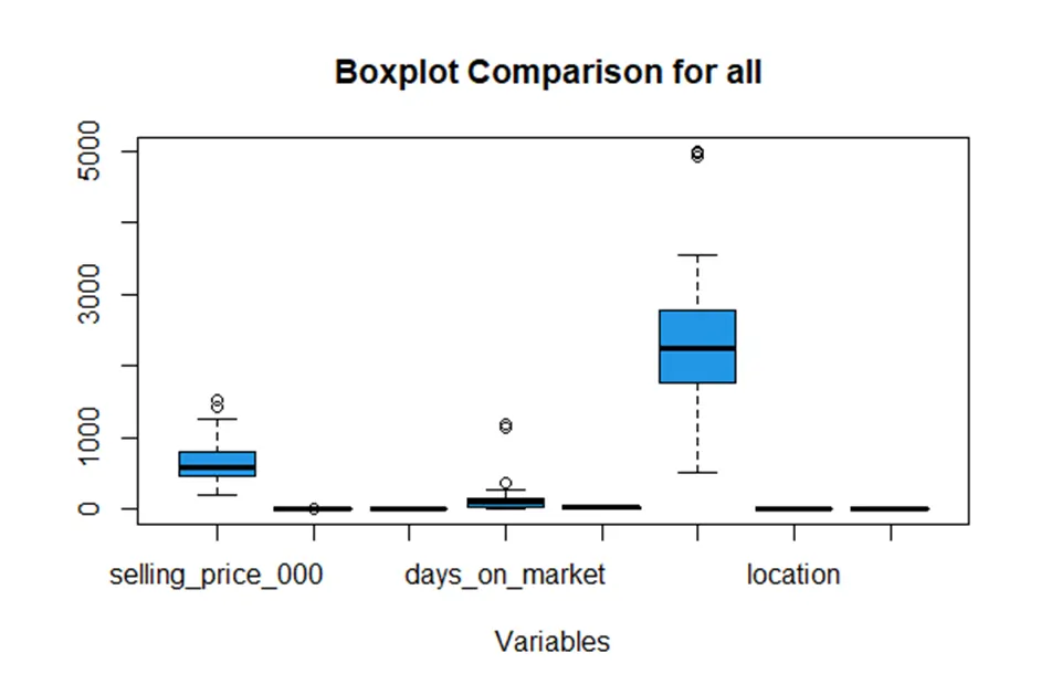
Boxplot
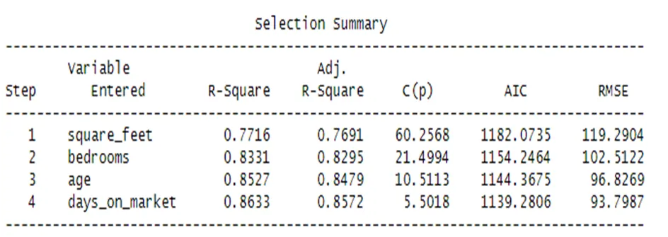
Model Fitting:
A multiple linear regression model was fitted to the data to predict the selling prices based on the selected attributes. The model was selected using a stepwise regression approach with a 5% significance level for variable inclusion. The chosen variables were square feet, bedrooms, age, and days on the market. These variables explained 85.7% of the variation in house selling prices.
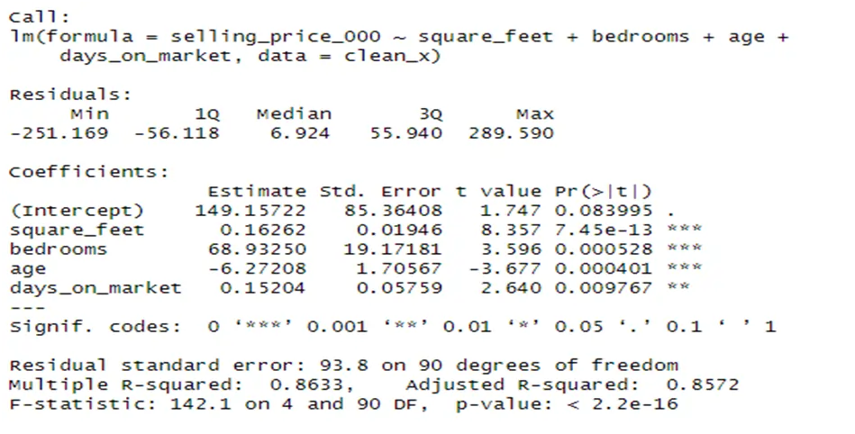
Conclusions:
The analysis concluded that square footage, number of bedrooms, and days on the market had a positive impact on house selling prices in Hollywood Beach, while the age of the house had a negative impact. Notably, the number of bedrooms had the most significant positive influence, accounting for up to 68% of the price fluctuations. On the other hand, each additional year of age reduced the average selling price by 6.3%.
R-Codes:
# Loading packages
install.packages("janitor")
install.packages("olsrr")
suppressPackageStartupMessages(library(dplyr))
suppressPackageStartupMessages(library(janitor))
suppressPackageStartupMessages(library(tidyverse))
suppressPackageStartupMessages(library(olsrr))
# Data set
data <- read.csv(file.choose())
view(data)
# Data Exploration and cleaning
str(data)
summary(data)
clean <- clean_names(data)
colnames(clean)
clean$location<- as.factor(clean$location)
clean$foreclosed<- as.factor(clean$foreclosed)
str(clean)
summary(clean)
# Checking for outliers
boxplot(clean,
main="Boxplot Comparison for all variables",
xlab="Variables",
col = 4)
clean_x<- clean %>% drop_na()
summary(clean_x)
for (x in c("selling_price_000","days_on_market"))
{
value = clean_x[,x][clean_x[,x] %in% boxplot.stats(clean_x[,x])$out]
clean_x[,x][clean_x[,x] %in% value] = NA
}
for (x in c("bedrooms","square_feet"))
{
value = clean_x[,x][clean_x[,x] %in% boxplot.stats(clean_x[,x])$out]
clean_x[,x][clean_x[,x] %in% value] = NA
}
clean_x<- clean %>% drop_na()
boxplot(clean_x,
main="Boxplot Comparison for all variables",
xlab="Variables",
col = 4)
view(clean_x)
# Regression model
model = lm(selling_price_000 ~ ., data = clean_x)
ols_step_forward_p(model, penter = 0.05)
Final_Model = lm(selling_price_000 ~ square_feet + bedrooms + age + days_on_market,
data = clean_x)
summary(Final_Model)