
Problem Description
This Data Analysis assignment focuses on conducting a regression analysis using data from a file named "prefixes.csv." The data includes reaction times (RT) and accuracy values for an auditory lexical decision task. The main goal is to prepare, analyze, and interpret the data to gain insights into the factors affecting reaction times.
Solution:
Data Preparation: Start by downloading the "prefixes.csv" file and loading it into R using read.csv(). We will begin by exploring the distribution of reaction times and address outliers.
R CODE:
# Data Loading
prefixes <- read.csv("prefixes.csv")
# Histogram of RT
library(rcompanion)
plotNormalHistogram(prefixes$RT)
# Log transformation of RT
prefixes$lRT <- log(prefixes$RT)
# Histogram of logRT
plotNormalHistogram(prefixes$lRT, xlab = "log of RT")
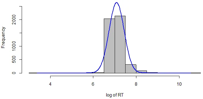
Fig 1: Histogram of logRT
Handling Outliers: To improve the data quality, we'll identify and remove outliers based on the mean and standard deviation of logRT.
- Mean of logRT: 7.092
- Standard Deviation of logRT: 0.35
We'll exclude RTs more than 3 standard deviations above or below the mean.
R CODE:
# Trimming outliers
prefixes_HR <- prefixes %>% filter(lRT < 8.141)
prefixes_LR <- prefixes_HR %>% filter(lRT > 6.043)
# Number of data points left
data_points_left <- nrow(prefixes_LR)
Improved Data Visualization: Create a histogram using the trimmed data to visualize the impact of outlier removal.
R CODE:
# Histogram of trimmed logRT
plotNormalHistogram(prefixes_LR$lRT, xlab = "Trimmed log of RT")
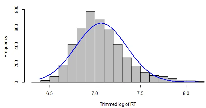
Fig 2: Histogram of Trimmed Log of RT
Regression Analysis: Perform a multiple regression analysis using the lm() function to predict logRT values from Lex, Age, and Sex.
R CODE:
# Multiple regression analysis
model <- lm(lRT ~ Lex + Age + Sex, data = prefixes_LR)
# Summary of the model
summary(model)
Model Summary: Present the model summary including estimates, t-values, and p-values for all factors.
R CODE:
# Model summary table
model_summary <- summary(model)
model_table <- data.frame(
Factor = rownames(model_summary$coefficients),
Beta_Estimate = model_summary$coefficients[, 1],
Std_Error = model_summary$coefficients[, 2],
T_Value = model_summary$coefficients[, 3],
P_Value = model_summary$coefficients[, 4]
)
R Script: Upload a copy of the R script for future reference.
R CODE:
# Your complete R script here
prefixes <- read.csv("prefixes.csv")
# ... (rest of the script)
Assignment 3B: Regression in the Wild (Summary): The article by Storkel (2004) investigates lexical acquisition in children and its relationship with word length, word frequency, and phonological neighborhood density. The analysis involves adult self-ratings of Age of Acquisition (AoA).
Interpretation of Results:
- Is the model a significant improvement over the null model?
Yes, the model is a significant improvement over the null model.
- How can you tell?
The statistical significance is determined by the F-statistic: F (5, 376) = 28.365, p < 0.001. The p-value being less than 0.001 suggests that the model is significantly better than the null model.
- Predictions of the Model:
Words in denser neighborhoods are acquired earlier than words with less dense neighborhoods.
Higher frequency words are acquired earlier than less frequent words.
Longer words are acquired later than shorter words.
- Most Statistically Significant Predictor:
Word frequency has the most statistically significant effect as it has the largest absolute t-value.