Enhancing Credit Scoring Through Statistical Analysis: A Case Study Using German Credit Data

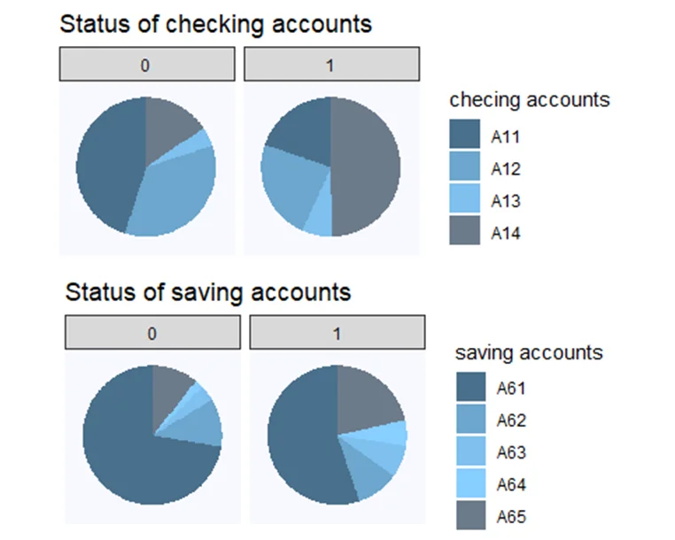
Fig 1: Categorical data visualization

Status of checking accounts:

The majority of clients classified as “good” have no checking accounts. It is an interesting remark - the intuition tells us that the higher balance of checking account is, the client is more likely to repay the loan on time. The description of the feature is rather vague so we can only speculate why the majority of “good” clients have no checking account.

We can also see that there are slight differences between two groups of clients who’s checking account balance is higher than zero. Respectively 16% and 11% of “good” and “bad” clients have 0-200 DM on their accounts. 5% of people paying back credits duly have more than 200 DM while within the group of “bad” clients there is only 1%.

Status of saving accounts:

Most of the clients classified as “good” have no saving account or the balance of their account is less than 100 DM. That observation is also surprising.

• Bivariate analysis explores differences between clients based on credit history, job, and other factors.

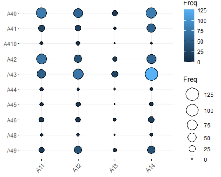
Fig 2: balloonplot from the ggplot package.

Purpose of loan and status of checking account

We can observe that there are no significant differences between clients grouped by the status of checking accounts. Customers mostly use their loans to buy the radio/television, car (new or used) or house equipment.

Loans are mostly for personal consumption (with given data). Therefore we can suppose that the median of the loan amount and the loan period in the given population should not be higher than respectively 3000 DM and 5 years. We can check this assumption by calculating some statistics.

Data Preprocessing:

• We check for missing values, finding none in our dataset.

The first step we should take in data preprocessing is to check whether there are any missing values in the dataset. To check if the German Credit dataset contains any missing values we will use the function “missmap” from the Amelia package.

checking_acc duration credit_history 0 0 0 purpose loan_amount saving_acc 0 0 0 employment_duration installment_in_income maritial_status 0 0 0 other_debtors residance properties 0 0 0 age other_installments housing_situation 0 0 0 existing_loans job maitaince 0 0 0 phone foregin_worker results 0 0 0 Dummy_results 0

• Outliers are detected and handled by replacing them with a mean ± 3 times the standard deviation.
• To address class imbalance, we oversample the data using the ROSE package.

over_data <-ovun.sample(Dummy_results ~ ., data = my_data, method ="over", N =1398)$data tab3 <-as.data.frame(table(my_data$Dummy_results)) colnames(tab3) <-c("Class", "Freq berfore oversampling") tab4 <-as.data.frame(table(over_data$Dummy_results)) colnames(tab4) <-c("Class", "Freq after oversampling") tab5 <-as.data.frame(cbind(tab3$Class, tab3$`Freq berfore oversampling`, tab4$`Freq after oversampling`)) colnames(tab5) <-c("Class", "Freq berfore oversampling", "Freq after oversampling") tab6 <- tab5 %>% formattable() tab6

Class

Freq berfore oversampling

Freq after oversampling

1

300

699

2

699

699

Splitting data into train and test

Now we can split the data into training and test

sample_data <-sample(nrow(over_data), 0.7*nrow(over_data)) train <- over_data[sample_data, ] test <- over_data[-sample_data, ] dim(train) [1] 978 22 dim(test) [1] 420 22

Correlation matrix

One of the assumptions of logistic regression is low correlation between independent variables. To check this assumption we will create the correlation matrix. To calculate correlation between variables of different types we can use a function “hetcor” from the polycor package.

train_corelation <-hetcor(train) train_cor_table <-as.data.frame(train_corelation$correlations) # install.packages('ggcorrplot') library(ggcorrplot) cor_plot1 <-ggcorrplot(train_cor_table, colors =c("azure1", "azure2", "lightcyan4", "cadetblue3")) +labs(title ="Correlation matrix") cor_plot1

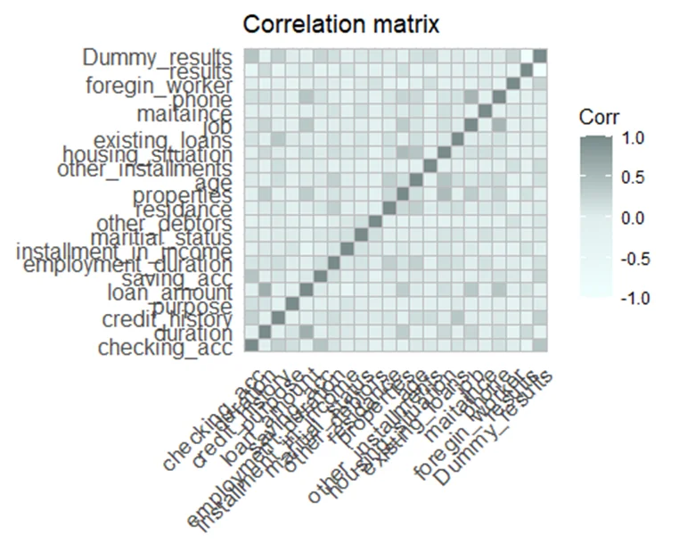
Fig 3: Correlation matrix

There is no strong correlation between any of variables from the German Credit Dataset.

Building the Logistic Regression Model:

• The logistic regression model is constructed using the glm() function, focusing on attributes like checking account status, saving account status, duration, age, and loan amount.

# Logistic regression model model1 <-glm(formula = Dummy_results ~ checking_acc + saving_acc + duration + age + loan_amount, data = train, family =binomial(link ="logit")) summary(model1) Call: glm(formula = Dummy_results ~ checking_acc + saving_acc + duration + age + loan_amount, family = binomial(link = "logit"), data = train) Deviance Residuals: Min 1Q Median 3Q Max -2.2217 -0.9513 0.4521 0.9359 1.9605 Coefficients: Estimate Std. Error z value Pr(>|z|) (Intercept) -8.288e-01 2.915e-01 -2.843 0.004472 ** checking_accA12 3.232e-01 1.835e-01 1.761 0.078181 . checking_accA13 6.698e-01 2.867e-01 2.337 0.019453 * checking_accA14 1.833e+00 1.933e-01 9.484 < 2e-16 *** saving_accA62 -7.230e-02 2.318e-01 -0.312 0.755105 saving_accA63 6.679e-01 3.786e-01 1.764 0.077728 . saving_accA64 6.331e-01 3.992e-01 1.586 0.112749 saving_accA65 6.828e-01 2.061e-01 3.312 0.000925 *** duration -3.057e-02 7.437e-03 -4.110 3.96e-05 *** age 2.010e-02 6.608e-03 3.041 0.002358 ** loan_amount 2.047e-06 3.282e-05 0.062 0.950254 --- Signif. codes: 0 '***' 0.001 '**' 0.01 '*' 0.05 '.' 0.1 ' ' 1 (Dispersion parameter for binomial family taken to be 1) Null deviance: 1354.6 on 977 degrees of freedom Residual deviance: 1140.4 on 967 degrees of freedom AIC: 1162.4 Number of Fisher Scoring iterations: 4 summary_model1_table <-summary(model1) model1_coeff <-as.data.frame(round(summary_model1_table$coefficients, 6)) # significance_function <- if() is_significant_fun <-function(x) { if (x >0.05) { "not significant" } else { "significant" } } model1_coeff$significance <-sapply(model1_coeff$`Pr(>|z|)`, is_significant_fun) model1_coeff Estimate Std. Error z value Pr(>|z|) significance (Intercept) -0.828759 0.291528 -2.842814 0.004472 significant checking_accA12 0.323159 0.183474 1.761337 0.078181 not significant checking_accA13 0.669838 0.286655 2.336738 0.019453 significant checking_accA14 1.833394 0.193319 9.483778 0.000000 significant saving_accA62 -0.072304 0.231808 -0.311915 0.755105 not significant saving_accA63 0.667908 0.378627 1.764025 0.077728 not significant saving_accA64 0.633097 0.399189 1.585958 0.112749 not significant saving_accA65 0.682757 0.206126 3.312332 0.000925 significant duration -0.030566 0.007437 -4.109806 0.000040 significant age 0.020095 0.006608 3.041042 0.002358 significant loan_amount 0.000002 0.000033 0.062388 0.950254 not significant

Interpreting the Coefficients:

• We interpret the coefficients of the model to understand how different features impact the probability of successful credit repayment.

For categorical variables we interpret the probability of success comparing the estimate of coefficient for particular level with the “reference level” (to set the reference level use the function relevel)

# Setting level for the feature checking account - I've set the reference level

# before building the model relevel(train$checking_acc, ref = 'less than 0 DM')

levels(train$checking_acc)

NULL

Example:

The reference level for the feature “status of checking account” is “less than 0 DM”. The positive value of estimates for the level “0-200 DM” (0.573706) means that a client having 0-200 DM on her/his checking account is more likely to pay back the loan on time compared to the client who has less than 0 DM on her/his account.

Output interpretation - AIC and null/residual deviance

AIC

AIC (Akaike information criterion) allows us to compare two models. Read more about AIC and BIC on Wikipedia: https://en.wikipedia.org/wiki/Akaike_information_criterion

The general rule is: choose the model with the lower value of AIC/BIC.

Null deviance/residual deviance

The lower the value of deviance is, the goodness of fit of the model is better. In glm() output for logistic regression null deviance shows how well fits the model which contains only the intercept. Residual deviance measures the goodness of fit for the model which includes all explanatory variables.

For the model we have built the value of the null deviance is 1354 whereas the value of residual deviance is 1139,7. It means that model containing explanatory variables could be characterized by better fitness than the model only with the intercept.

Model Validation: Confusion Matrix

Confusion matrix presents how many of predictions are: * true positive, * true negative, * false positive, * false negative.

Building the confusion matrix is a great method to check the accuracy of the model. In R language there is a dedicated function confusionMatrix() - however we can also build the confusion matrix with a function table(). We will compare the predictions of the built model with the test subset of data.

# Confusion matrix predicted <-predict(model1, newdata = test, type ="response") pred <-ifelse(predicted >0.5, 1, 0) table(predicted = pred, actuals = test$Dummy_results) actuals predicted 0 1 0 175 74 1 52 119

Conclusions

In this study, we have successfully delved into the world of Credit Scoring using real-world data from the German Credit Dataset. By employing logistic regression, we have created a model that aids decision-makers in streamlining the credit assessment process, making it more efficient and less prone to human errors. The insights gained from this analysis can pave the way for future improvements, including the implementation of advanced techniques such as ensemble methods and deep learning models to further enhance credit scoring accuracy.