
Problem Description:
The data analysis assignment at hand involves analyzing a dataset named "25_4m_priming.jmp" that contains valuable information for a courier service company. The dataset includes three key variables:
- Y Variable: Number of courier parks used after the promotion.
- X Variable: Amount of time spent with the client by the sales representative.
- D Variable: Indicates whether or not the customer had been aware of the courier parks prior to the visit.
The assignment consists of various questions that aim to explore the relationship between client interaction time, customer awareness, and the number of courier parks used after a promotional visit.
Let's dive into the key insights and findings from the assignment:
Question 1: Dataset Description
In the provided dataset, we have information on the number of courier parks used, the time spent with clients, and their awareness of courier parks. This data forms the foundation for our analysis.
Question 2: ANCOVA Model
We employ an ANCOVA model to investigate the impact of client interaction time and awareness on courier parks usage. The ANCOVA model is expressed as:
Y = β0 + β1 * Hours + β2 * Aware + β3 * Hours * Aware + ε
Where:
- β0 is the intercept.
- β1 represents the coefficient of the continuous independent variable (Hours).
- β2 represents the coefficient of the categorical independent variable (Aware).
- β3 accounts for the interaction effect between Hours and Aware.
- ε denotes the error term.
The model is further detailed as follows:
Y = 2.45 + 13.82 * Hours + 1.71 * Aware + 4.31 * Hours * Aware + ε
Interpretation of coefficients:
- β0 represents the estimated value of mailings when hours and awareness are both zero.
- β1 signifies the change in Y for a unit change in Hours, with awareness held constant.
- β2 represents the change in Y for a unit change in awareness, with hours held constant.
- β3 captures the interaction effect between hours and awareness on mailings.
Question 3:

Question 4: Statistical Significance of Variables
After constructing the regression model, we examine the Parameter Estimates panel to assess the statistical significance of the variables. In our case, the hours of effort and the interaction term appear to be statistically significant, while the dummy variable (awareness) does not carry statistical significance.
Question 5: Hypothesis Testing
The p-value for the test H0: R^2 = 0 vs. H1: R^2 ≠ 0 is 0.00. This low p-value indicates that there is substantial evidence to reject H0 if p-value < 0.05.
Question 6: The Principle of Marginality
The principle of marginality is a crucial aspect in multiple regression models. If an interaction term is included, the main effects for the variables involved in the interaction term should also be included. This ensures a comprehensive analysis, even if these main effects are not statistically significant individually. The presence of an interaction term can influence the interpretation of the main effects, making their inclusion necessary to avoid biased or misleading results.
Question 7: The Final ANCOVA Model
The final fitted ANCOVA model is presented as:
mailings = 3.12 + 13.57 * Hours + 4.926 * Hours * Aware
The model's goodness of fit is measured through R^2, which is 0.76618, indicating that the model explains approximately 76.62% of the variance in the dependent variable. Additionally, the adjusted R^2 is 0.7623, and the RMSE (root mean square error) is 11.12591, which assesses the model's prediction accuracy.
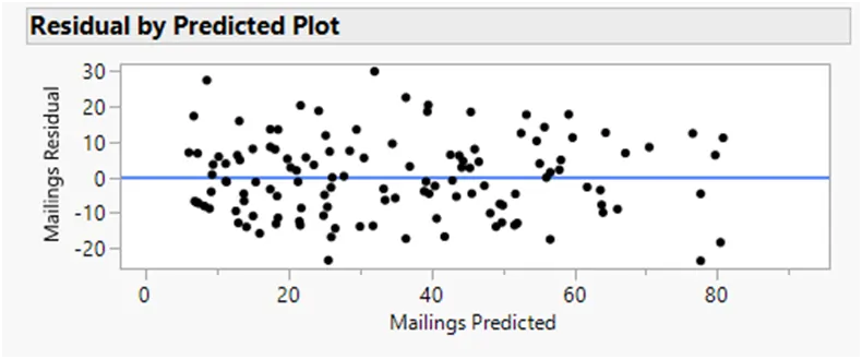
Question 8: Assumption of Constant Variance
We evaluate the constant variance assumption by examining the residual plot generated by JMP. The plot shows that residuals are randomly scattered around the horizontal axis, with no discernible pattern or change in the spread of residuals across different levels of the predictor variable(s). The mean of the residuals is 0, supporting the assumption that the model's errors have constant variance. Hence, the constant variance assumption seems to hold for this dataset.
Question 9: Normal Distribution Assumption
The normal distribution assumption is evaluated through the inspection of a normal quantile plot (Q-Q plot) produced by JMP.
Question 10:
For a typical hour of contact with a follow-up sales representative, the number of shipments generated for clients who were aware of Courier Parks is estimated to be 21.65.
Question 11: Impact of Interaction
Assuming the parameter estimates are independent, it appears that follow-up visits are less effective for customers who were already aware and had spent 3 hours, as the mailings for 3 hours are greater than those for just one hour of contact.