
Problem Description:
This MINITAB assignment consists of multiple questions covering various statistical and data analysis topics. Here, we present a structured and organized presentation of the solutions for each question.
Solution
Question 1 – Salary Sheet
Identify the type of each parameter (Qualitative & Quantitative).
Job level, sector, education, and discipline are qualitative parameters because these parameters cannot be measured in terms of numeric and have distinct qualities. For instance, the sector has two distinct qualities i.e., public and private. Age, salary, and customer satisfaction are quantitative parameters because these parameters can be measured and expressed in numeric terms.
Create summary table for Job Level.
Most of the respondents were working at the senior level (44.57%). Likewise, a similar proportion of the respondents were working at the manager level (43.26%). A few respondents were also working at the junior level (12.17%).
Table 1 – Summary Table for Job Level
| Job Level | Count | % of Total |
|---|---|---|
| Junior | 83 | 12.17% |
| Manager | 295 | 43.26% |
| Senior | 304 | 44.57% |
| Total | 682 | 100.00% |
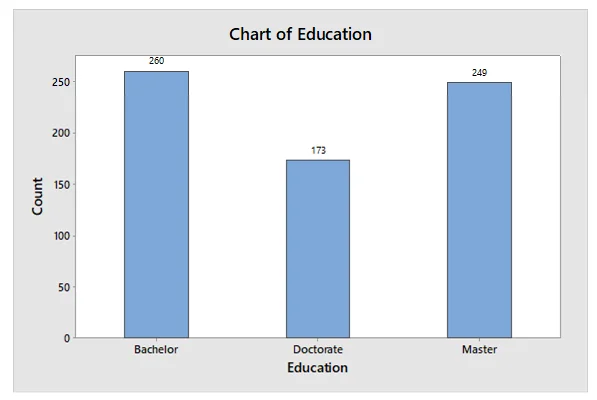
Draw bar graph for Education.
The bar graph for Education indicated that most of the respondents hold either Bachelor’s degree or a Master’s degree. A small proportion of respondents also hold a Doctorate degree.
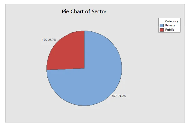
Draw pie chart for Sector.
The pie chart indicated that in terms of sector, almost three-fourth of the respondents were working in the private sector (74.3%), while 25.7% of respondents were working in the public sector.
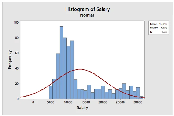
Draw a histogram for salary.
The histogram for salary indicated that most of the respondents had a salary of around $5,000 to $125,000. It also indicated that the distribution of salary is not normal because most of the values fell on the right side of the histogram.
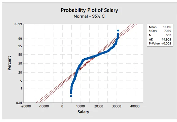
Calculate descriptive statistics of Salary and test its normality
The descriptive statistics of Salary indicated that the average salary of the sample is $13,310 with a variability of $7,039. The salary ranges from $4,830 to $30,534. The skewness of the salary is 1.07, and the kurtosis of the salary is −0.17. Since the values fell outside the acceptable threshold (Skewness/ Kurtosis threshold: −1 to +1) which indicated that the distribution of salary is not normal. The normal P-P plot also indicated that the value of Anderson-Darling (AD) is significant at 5% (AD = 44.905, p < 0.05), which inferred that the salary is not normally distributed.
Descriptive Statistics: Salary
Variable N N* Mean SE Mean StDev Minimum Q1 Median Q3 Maximum
Salary 682 0 13310 270 7039 4830 8171 10471 17581 30534
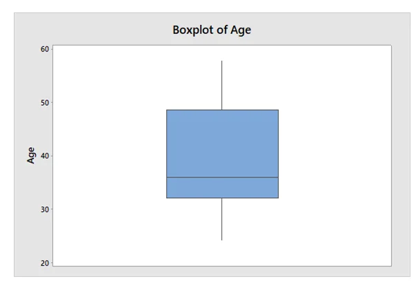
Draw box plot for Age and determine the existence of outliers
The box plot of age indicated that the average age of the sample is 35 years. Some respondents are also old in age i.e., around 40 years to 50 years. The box plot did not detect the existence of outliers.
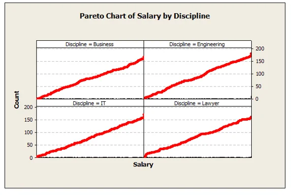
Draw a Pareto chart for total salary of each Discipline & present your conclusion about the vital few
The Pareto chart for the total salary of discipline indicated that the salary of engineering personal are higher compared to the salary of business personal, which are even higher compared to IT and lawyer personal.
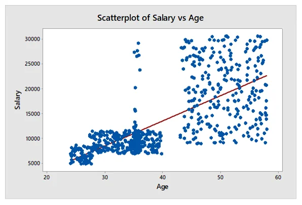
Draw a scatter diagram between Age & Salary and discuss the result to obtain conclusion about the relationship between the two parameters.
The scatter diagram between age and salary indicated that there is a positive relationship between age and salary. The R2 indicated that 50.8% of variation in salary can be explained by age. Hence, it can be inferred that as a person gets older, the salary also increases because they have more experience with age. The regression equation for salary is given as:
Salary = −6834 + 507.3*Age
Question 2 – Probability
1. You are working in TV set factory. The manufactured TV has a normal distribution life with = 3,500 working hours and = 200 hours.
- What is the probability that a TV will work less than 3,350 hours?
The probability that a TV will work less than 3,350 hours is
P (X<3350)=P ((X- μ)/σ< (3350-3500)/200)
P (X<3350)=P (Z< (-150)/200)
P (X<3350)=P (Z<-0.75)
Using the Excel formula for normal distribution ‘NORM.S.DIST(−0.75, TRUE), we get
P (X<3350)=P (Z<-0.75)= 0.2266
Hence, the probability that a TV will work less than 3,350 hours is 0.2266 or 22.66%.
- What is the probability that a TV will work more than 3,750 hours?
The probability that a TV will work more than 3,750 hours is
P (X>3750)=1-P ((X- μ)/σ< (3750-3500)/200)
P (X>3750)=1-P (Z< 250/200)
P (X>3750)=1-P (Z<1.25)
Using the Excel formula for normal distribution ‘NORM.S.DIST(1.25, TRUE)’, we get
P (Z<1.25)= 0.8944
Using this value,
P (X>3750)=1-0.8944=0.1054
Hence, the probability that a TV will work more than 3,750 hours is 0.1054 or 10.54%.
- What is the probability that a TV will work between 3,350 & 3,750 hours?
The probability that a TV will work between 3,350 & 3,750 hours is
P (3350
P (3350
From the previous parts, the probability values were taken as:
P (3350
P (3350
Hence, the probability that a TV will work between 3,350 & 3,750 hours is 0.6678 or 66.78%.
- What is TV life that you are confident 95% it will keep working?
The TV life at which 95% confident is achieved that it will keep working can be calculated as:
X= μ+Zσ
Considering z-score at 95% confidence level be −1.645, μ be 3500, and σ be 200, the TV life (X) can be calculated as:
X=3500+(-1.645 ×200)
X=3171
Hence, the TV life at which 95% confident is achieved that it will keep working is 3,171 hours.
2. You are working in a bank. You have collected enough data to determine the average time needed to serve one customer and found that it follows a normal distribution with = 4.78 minutes and = 1.32 minutes.
- What is the probability that you will serve 10 customers every hour?
Since 10 customers are to serve in every hour i.e., 60 minutes, each customer will be served in an average of 6 minutes. Considering this average time, the probability that you will serve 10 customers every hour is
P (X=6)=P ((X- μ)/σ= (6-4.78)/1.32)
P (X=6)=P (Z= 1.22/1.32)
P (X=6)=P (Z=0.92)=0.3212
Hence, the probability that you will serve 10 customers every hour is 0.3212 or 32.12%.
- What is the probability that you will serve more than 15 customers every hour?
Since 15 customers or more are to serve in every hour i.e., 60 minutes, each customer will be served in an average of 4 minutes. The probability that you will serve more than 15 customers every hour is
P (X>4)=1-P ((X- μ)/σ< (4-4.78)/1.32)
P (X>4)=1-P (Z< (-0.78)/1.32)
P (X>4)=1-P (Z<-0.59)
Using the Excel formula for normal distribution ‘NORM.S.DIST(−0.59, TRUE)’, we get
P (Z<-0.59)= 0.2776
Using this value,
P (X>4)=1-0.2776=0.7226
Hence, the probability that you will serve more than 15 customers every hour is 0.7226 or 72.26%.
- What is the probability that you will serve between 10 & 15 customers every hour?
Finding the probability of serving between 10 and 15 customers every hour means the probability of serving between average time of 4 and 6 minutes per customers. The probability that you will serve between 10 & 15 customers every hour is
P (4
P (4
P (4
Hence, the probability that you will serve between 10 & 15 customers every hour is 0.4014 or 40.14%.
- What is the number of customers you will be 95% confident that you will serve every hour?
The number of customers at which 95% confident is achieved that you will serve every hour can be calculated as:
X= μ+Zσ
Considering z-score at 95% confidence level be −1.645, μ be 4.78, and σ be 1.32, the number of customers (X) can be calculated as:
X=4.78+(-1.645 ×1.32)
X=2.61 ~ 3
Hence, the number of customers at which 95% confident is achieved that you will serve every hour is 3 customers.
3. You are thinking about signing a contract, as a supplier for one of the biggest global exporting company. The draft contract obligates you to deliver 20 tons of orange every week. The delivery process of orange during this season follows a normal distribution with = 22.5 tons every week and = 3.2 tons.
- What is the probability that you will achieve the contract terms?
The probability that you will achieve the contract terms is
P (X<20)=P ((X- μ)/σ< (20-22.5)/3.5)
P (X<20)=P (Z< (-2.5)/3.5)
P (X<20)=P (Z<-0.71)
Using the Excel formula for normal distribution ‘NORM.S.DIST(−0.71, TRUE), we get
P (X<20)=P (Z<-0.71)= 0.2389
Hence, the probability that you will achieve the contract terms is 0.2389 or 23.89%.
- What is the orange quantity that you will be 95% confident that you will deliver every week?
The orange quantity at which 95% confident is achieved that you will deliver every week can be calculated as:
X= μ+Zσ
Considering z-score at 95% confidence level be −1.645, μ be 22.5, and σ be 3.5, the orange quantity (X) can be calculated as:
X=22.5+(-1.645 ×3.5)
X=16.74 ~ 17
Hence, the orange quantity at which 95% confident is achieved that you will deliver every week is 17 oranges.
Question 3 – Customer Survey
- Check if customer satisfaction of Product A is less than 3.
One-sample t-test is conducted to determine if the customer satisfaction of Product A is less than 3. Results indicated that the t-value is not significant at 5% level (t = 3.57, p = 1.00). Hence, it can be concluded that the customer satisfaction of Product A is not less than 3. The mean score for the customer satisfaction of Product A is calculated as 4.978, which is higher than hypothesized mean i.e., 3.
Table 2 – One-Sample t-test for Customer Satisfaction of Product A
| t-test | N | Mean | Standard Deviation | t-value | p-value |
|---|---|---|---|---|---|
| Customer Satisfaction (A) | 46 | 4.978 | 3.762 | 3.57 | 1.000 |
- Check if there is a significant difference between Product A & Product B customer satisfaction.
Independent-sample t-test is conducted to determine if there is a significant difference between Product A & Product B customer satisfaction. Firstly, equality of variances was tested by Levene’s test and found that customer satisfaction of both Product A and Product B has equal variances (F (1) = 3.66, p = 0.059). Hence, computing independent-sample t-value while assuming equal variances, results indicated that t-value is not significant at 5% level (t (90) = 0.55, p = 0.587). Hence, it can be concluded that there is no significant difference between Product A & Product B customer satisfaction. The mean scores for the customer satisfaction of Product A and Product B are calculated as 4.98 and 4.59 respectively, which is almost same for both products.
Table 3 – Independent-Sample t-test for Customer Satisfaction of Product A & Product B
| Product A M (SD) |
Product B M (SD) |
Levene’s Test F (p) |
Independent t-test t (p) |
|
|---|---|---|---|---|
| Customer Satisfaction | 4.98 (3.76) | 4.59 (3.09) | 3.66 (0.059) | 0.55 (0.587) |
- Check if there is a significant difference between Product B & Product C customer satisfaction.
| Product B M (SD) |
Product C M (SD) |
Levene’s Test F (p) |
Independent t-test t (p) |
|
|---|---|---|---|---|
| Customer Satisfaction | 4.59 (3.09) | 4.72 (2.86) | 0.26 (0.612) | −0.21 (0.832) |
Question 4 – Fuel Consumption Data
- Study the relationship between fuel consumption per kilometer and the car speed using scatter diagram and correlation coefficient.
The scatter diagram below indicated that there is a negative relationship between the fuel consumption per kilometer and the car speed. The correlation coefficient is calculated as −0.66 and is significant at 1% (r = −0.66, p <0.01), which further concluded that there is a strong negative relationship between the fuel consumption per kilometer and the car speed.
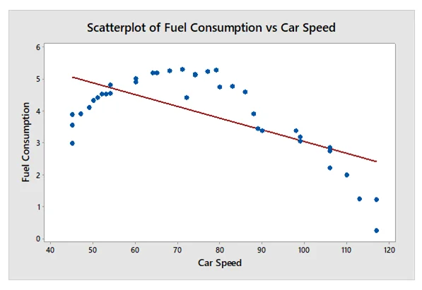
- Develop a mathematical equation to predict the fuel consumption per kilometer using car speed. The mathematical equation to predict the fuel consumption per kilometer using car speed is given as:
Fuel Consumption = 6.738 – 0.037*Car Speed
- Develop your conclusion based on the studied relationship.
Considering the scatterplot, correlation coefficient, and slope of regression equation, the inferences is correctly made i.e., there is a strong negative relationship between fuel consumption per kilometer and car speed.
- Provide your comments on the prediction accuracy of this equation.
The prediction accuracy of this equation can be determined by the coefficient of determination (R2), which is calculated to be 44.4%. This indicated that 44.4% of variation in fuel consumption per kilometer can be explained by car speed.
- Predict the car fuel consumption, if the car speed is 100 km/hour.
The car fuel consumption, if the car speed is 100 km/hour, can be calculated as:
Fuel Consumption = 6.738 – 0.037*Car Speed
Fuel Consumption = 6.738 – 0.037*100
Fuel Consumption = 6.738 – 3.7
Fuel Consumption = 3.038
Hence, the car fuel consumption, if the car speed is 100 km/hour is 3.038 liters per kilometer.
Question 5 – Labor Production Data
- Develop a mathematical equation to predict the labor production using all factors.
The mathematical equation to predict the labor production using all factors is
Production (kg) = 281.2 – 0.467*Age – 13.786*Temp + 2.521*Exp + 1*(Shift A) – 1.91*(Shift B) – 3.87*(Shift C)
- Provide your comments on the prediction accuracy of the previous equation.
The prediction accuracy of this equation can be determined by the coefficient of determination (R2), which is calculated to be 93.64%. This indicated that 93.64% of variation in labor production can be explained by age, temperature, experience, and three shifts.
- Develop a mathematical equation to predict the labor production using two factors only.
The mathematical equation to predict the labor production using two factors only is
Production (kg) = 343.1 – 15.25*Temp + 2.395*Exp
- Provide your comments on the prediction accuracy of the previous equation.
The prediction accuracy of this equation can be determined by the coefficient of determination (R2), which is calculated to be 90.36%. This indicated that 90.36% of variation in labor production can be explained by temperature and experience.
Question 6 – Call Center
Call agent experience (Moderate or High), - Type of customer request (Simple or Complex) - System used by the call agent to record request (Manual or Automated)
- Establish a Full Factorial Design for the above mentioned case, using one replicate without center point.
The Full Factorial Design for the above-mentioned case, using one replicate without center point is:
| StdOrder | RunOrder | CenterPt | Blocks | Call agent experience | Type of customer request | System used by the call agent to record request |
|---|---|---|---|---|---|---|
| 6 | 1 | 1 | 1 | High | Simple | Manual |
| 1 | 2 | 1 | 1 | Moderate | Simple | Automated |
| 4 | 3 | 1 | 1 | High | Complex | Automated |
| 3 | 4 | 1 | 1 | Moderate | Complex | Automated |
| 7 | 5 | 1 | 1 | Moderate | Complex | Manual |
| 2 | 6 | 1 | 1 | High | Simple | Automated |
| 5 | 7 | 1 | 1 | Moderate | Simple | Manual |
| 8 | 8 | 1 | 1 | High | Complex | Manual |
- How many runs we need to perform, if we decided to conduct Half Factorial.
4 runs we need to perform, if we decided to conduct Half Factorial. The Half Factorial Design for the above-mentioned case, using one replicate without center point is:
| StdOrder | RunOrder | CenterPt | Blocks | Call agent experience | Type of customer request | System used by the call agent to record request |
|---|---|---|---|---|---|---|
| 1 | 1 | 1 | 1 | Moderate | Simple | Automated |
| 2 | 2 | 1 | 1 | Moderate | Complex | Manual |
| 3 | 3 | 1 | 1 | High | Simple | Manual |
| 4 | 4 | 1 | 1 | High | Complex | Automated |
- What is your conclusion on the resolution of the previous Half Factorial design.
The Half Factorial design is created on Resolution III, in which some main effects are confounded with two-way interactions. This design is defined relation for a 2k-p fractional factorial i.e., 23-1 or 4 runs.