
Problem Description
In this SAS assignment, we aim to investigate whether a high school student's Grade Point Average (GPA) can be predicted based on their ACT scores. This involves a comprehensive statistical analysis. The central question is: Can we reliably predict GPA from ACT scores? To address this question, we will perform various statistical tests and analyses.
Part I: Confidence Interval for Slope (β_1)
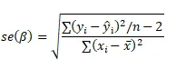
To begin, we calculate the confidence interval for the slope (β_1) with a 99% confidence level. This confidence interval helps us understand the range within which we can expect the true slope of the regression to lie. The calculation involves the standard error of the slope (se(β_1)).
The confidence interval for β1
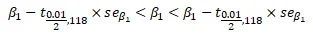
Where:
The results are as follows:
| Parameter Estimates | ||||||||
|---|---|---|---|---|---|---|---|---|
| Variable | Label | DF | ParameterEstimate | StandardError | t Value | Pr > |t| | 99% Confidence Limits | |
| Intercept | Intercept | 1 | 2.11405 | 0.32089 | 6.59 | <.0001 | 1.27390 | 2.95420 |
| ACT | ACT | 1 | 0.03883 | 0.01277 | 3.04 | 0.0029 | 0.00539 | 0.07227 |
Table 1: Parameter Estimates Table
Interpretation: The 99% confidence interval for the slope (β_1) is between 0.00539 and 0.07227. This means we are 99% confident that, for the population, a one-unit increase in ACT scores will result in a GPA increase within this range.
Part II: Hypothesis Testing for Significance of ACT on GPA
We formulate the following hypotheses:
- Null Hypothesis (H0): β_1 = 0 (ACT has no significant effect on GPA).
- Alternative Hypothesis (H1): β_1 ≠ 0 (ACT has a significant effect on GPA).
The test statistic (t) is calculated as follows:

| Test Statistics | |
| t | 3.04 |
Table 2: Test Statistics
Decision Rule: If the test statistic is greater than the critical value (t0.01/2, 118), we reject the null hypothesis. The critical value at the 1% significance level is 2.618.
Conclusion: The test statistic (3.04) is greater than the critical value (2.618), so we reject the null hypothesis. This indicates that ACT scores have a significant effect on GPA.
Part III: P-Value Interpretation
The p-value for this test is 0.0029. A p-value less than the significance level (0.01) leads to the rejection of the null hypothesis. This p-value aligns with our previous hypothesis test, providing further evidence that ACT scores significantly affect GPA.
Part IV: Confidence Interval and Prediction Interval for ACT = 28
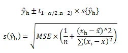
Next, we calculate the 95% confidence interval for the GPA of students with an ACT score of 28. The confidence interval is:
Y ̂_h interval equation
| Predicted Value | Std Error | 95% Confidence Limits |
|---|---|---|
| 3.2012 | 0.0706 | 3.0614 to 3.341 |
Table 3: 95% Confidence Limits Table (for confidence interval)
Interpretation: We are 95% confident that the average GPA for students with an ACT score of 28 in the population lies between 3.0614 and 3.341.
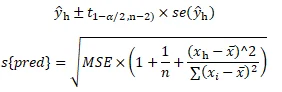
Additionally, we calculate a 95% prediction interval for an individual student with an ACT score of 28, resulting in the following interval:
| Predicted Value | Std Error | 95% Prediction Limits |
|---|---|---|
| 3.2012 | 0.0706 | 1.9594 to 4.4431 |
Table 4: 95% Prediction Limits Table (for prediction interval)
Interpretation: We are 95% confident that an individual's GPA, given an ACT score of 28, will fall within the range of 1.9594 to 4.4431.
Part V: Comparison of Confidence and Prediction Intervals
It's important to note that the prediction interval is wider than the confidence interval, as the prediction interval accounts for individual variation, including the error term (MSE).
Part VI: Plot Analysis
A plot illustrating the fit line with the confidence interval demonstrates that the confidence interval is relatively narrow, suggesting low uncertainty in the prediction.
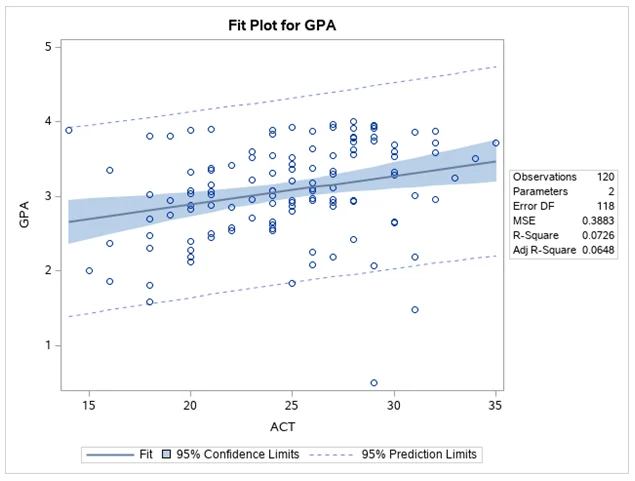
Fig 1: Fit Plot for GPA
Part VII: ANOVA (Analysis of Variance)
An ANOVA analysis was conducted to assess the overall significance of the model. The results are as follows:
| Source | DF | Sum of Squares | Mean Square | F Value | Pr > F |
|---|---|---|---|---|---|
| Model | 1 | 3.58785 | 3.58785 | 9.24 | 0.0029 |
| Error | 118 | 45.81761 | 0.38828 | ||
| Total | 119 | 49.40545 |
Table 5: Analysis of Variance Table
This analysis confirms that the model is statistically significant, with a small p-value (0.0029), indicating a significant relationship between ACT scores and GPA.
Part VIII: MSR and MSE
MSR (Mean Square due to Regression) and MSE (Mean Square due to Error) were discussed. These metrics help in understanding the variance explained by the model and the unexplained variance, respectively.
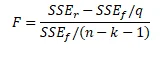
Part IX: Hypothesis Testing Using F-Test
We conducted an F-test to assess the significance of β_1. The results are as follows:
| Test Statistics | |
| F | 9.24 |
Table 6: Test Statistics Table
Decision Rule: If F-calculated (9.24) is greater than the critical value of F at the 1% significance level and (1, 118) degrees of freedom (6.58), we reject the null hypothesis.
Conclusion: We conclude that β_1 is significantly different from 0, indicating a significant linear relationship between ACT scores and GPA.
Part X: R-squared Interpretation
The absolute magnitude of the reduction in the variation of Y when X (ACT) is introduced into the regression model is 3.588. The relative magnitude, R-squared, is calculated as 0.0726.
The null and alternative hypothesis is

The test statistics is given by
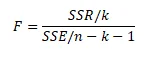
The test statistics value is 9.24
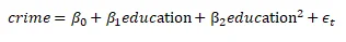
Part XI: Second Question - Crime Rate and Education
In the second part of the assignment, we analyze the relationship between crime rate and education, focusing on a full model and a reduced model. We perform ANOVA tests to determine the significance of the relationship between crime rate and education.
r=√0.0726
r=+0.27
Q2
The full model is
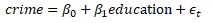
The reduced model is
Full Model
| Analysis of Variance | |||||
|---|---|---|---|---|---|
| Source | DF | Sum ofSquares | MeanSquare | F Value | Pr > F |
| Model | 2 | 99107366 | 49553683 | 8.93 | 0.0003 |
| Error | 81 | 449628742 | 5550972 | ||
| Corrected Total | 83 | 548736108 | |||
Table 7: Analysis of Variance – Full Model
Reduced Model
| Analysis of Variance | |||||
|---|---|---|---|---|---|
| Source | DF | Sum ofSquares | MeanSquare | F Value | Pr > F |
| Model | 1 | 93462942 | 93462942 | 16.83 | <.0001 |
| Error | 82 | 455273165 | 5552112 | ||
| Corrected Total | 83 | 548736108 | |||
Table 8: Analysis of Variance- Reduced Model
SSE(F)= 449628742
SSE(R) = 455273165
DF(F)=n-k-1=84-2-1=81
DF(R)=n-k-1=84-1-1=82
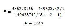
Decision rule: if the F-stat is less than critical value of F at 1% significance level and (1,81) df, we reject the null hypothesis. Since the F-stat (1.017) is less than the critical value (6.96) we cannot reject the null hypothesis that the relationship between crime rate and percentage of high school graduates is not linear. We conclude that a linear relationship between crime rate and percentage of high school graduates.
Code:
The provided code is used for regression analysis, plotting, and ANOVA tests. It serves as the practical implementation of the statistical analyses discussed in the assignment.
im proc reg data=WORK.IMPORT2 alpha=0.01 plots(only)=(diagnostics residuals
fitplot observedbypredicted);
model GPA=ACT / clb;
run;
quit;
data c;
input ACT;
cards;
28
;
data new;
set WORK.IMPORT2 c;
run;
proc reg data=new plots=(NONE);
model GPA=ACT/clm cli;
output out=Pred p=P; /* predicted values for the scoring data */
quit;
proc print data=Pred;
run;
proc reg data=WORK.IMPORT2 alpha=0.05 plots(only)=(diagnostics residuals
fitplot observedbypredicted);
model GPA=ACT / clb;
run;
quit;
/*2*/
proc reg data=WORK.IMPORT4 alpha=0.01 plots(only)=(diagnostics residuals
fitplot observedbypredicted);
model Crime=Edu / clb;
run;
quit;
proc glmselect data=WORK.IMPORT4 outdesign(addinputvars)=Work.reg_design;
model Crime=Edu Edu*Edu / showpvalues selection=none;
run;
proc reg data=Work.reg_design alpha=0.01 plots(only)=(diagnostics residuals
observedbypredicted);
ods select ParameterEstimates DiagnosticsPanel ResidualPlot
ObservedByPredicted;
model Crime=&_GLSMOD / clb;
run;
quit;
proc delete data=Work.reg_design;
run;
Conclusion
In conclusion, this assignment explores the intricate relationship between variables, especially the impact of ACT scores on GPA. The analyses and results provide a comprehensive understanding of how statistical tools can be utilized to make informed predictions and decisions